Data Analysis in R

Josh Allen

Department of Political Science at Georgia State University

10/7/22

Research Data Services

Our Team

Also, we do not have the capacity to provide pre-scheduled frequent software tutoring that is divorced from a specific assignment or software troubleshooting task at hand – in other words, we are also not generalized software tutors.

Our one-on-one software assistance is available to help you troubleshoot specific tasks or assignments. If you are seeking generalized software help, we direct you to our live workshops and our recorded workshops to gain the foundational skills for using various analytical software. Then, when or if the time comes that you have targeted software questions or specific issues to tackle related to a course assignment or research project, please feel free to contact us for one-on-one support.

Get Ready Badges

https://research.library.gsu.edu/dataservices/data-ready

These are awesome to share on social media i.e. linkedin which is a good signal to potential employers that you know this stuff

How To Get the Badges

Packages You Will Need

install.packages("pacman")

pacman::p_load("sandwich", # standard error fixes
               "lmtest", # diagnostic tests
               "marginaleffects", # getting marginal effects
                "emmeans", # getting marginal effect
                 "modelsummary", # making tables 
                 "broom", # pull diagnostic statistics
               "caret", # lots of machine learning  models
                "tidyverse", # ggplot and friends 
                 "fixest", # fixed effects 
                 "kableExtra", # extenstions for making latex tables
                  "plm",  # panel data models 
                  "ggfortify", install = TRUE)

set.seed(1994) # some of the models we will 

# data we are using
penguins = palmerpenguins::penguins 

Note this workshop is not a workshop that will teach you how these methods work. I presume that most of you will be familiar with linear regression and maximum likelihood estimation. If any of you are here with more of a machine learning background this includes logit and what not.

I also assume you know the basics of indexing I will go through a bit of it but you should probably know that before doing data analysis

This workshop is going to sort of through building the results section of a paper. This will generally be geared toward a social science audience. But the fundamentals are virtually the same if you are not.

Exploratory Data Analysis in R

Describing Variables

• This depends on what kind of variable it is i.e. continuous, categorical etc

• It also depends on what story you need to tell

  • Is this confounder a big deal?
  • Do we see anticipation of treatment?
  • Are there any outliers?
  • etc?

• Remember R is just a toolbox.

Exploratory data analysis is the first step of any data analysis pipeline. You need to understand your data in order to understand how to handle things. What does the distribution look like of your outcome variable. If you are like me and ended up taking a lot of causal inference classes and or read a lot of causal inference papers lots of the first parts of papers are just presenting EDA results to convince the reader that the assumptions are met.

Today we will be asking what is the relationship between bill length and body mass

hopefully that seems like a sensible research question. If not well the goal is just to show you how to generate descriptive statistics in R

First Cut

summary(penguins) 

      species          island    bill_length_mm  bill_depth_mm  
 Adelie   :152   Biscoe   :168   Min.   :32.10   Min.   :13.10  
 Chinstrap: 68   Dream    :124   1st Qu.:39.23   1st Qu.:15.60  
 Gentoo   :124   Torgersen: 52   Median :44.45   Median :17.30  
                                 Mean   :43.92   Mean   :17.15  
                                 3rd Qu.:48.50   3rd Qu.:18.70  
                                 Max.   :59.60   Max.   :21.50  
                                 NA's   :2       NA's   :2      
 flipper_length_mm  body_mass_g       sex           year     
 Min.   :172.0     Min.   :2700   female:165   Min.   :2007  
 1st Qu.:190.0     1st Qu.:3550   male  :168   1st Qu.:2007  
 Median :197.0     Median :4050   NA's  : 11   Median :2008  
 Mean   :200.9     Mean   :4202                Mean   :2008  
 3rd Qu.:213.0     3rd Qu.:4750                3rd Qu.:2009  
 Max.   :231.0     Max.   :6300                Max.   :2009  
 NA's   :2         NA's   :2                                 

If we just want like the quickest and dirtiest look at all the variables in our data we can use summary. Functionally this works because palmerpenguins is a small toy dataset. Thankfully for me we can access the raw data that the penguins dataset is based on. This is just the penguins raw function in the palmer penguins packagte.

Summary with a bigger data frame

penguins_bigger = palmerpenguins::penguins_raw

summary(penguins_bigger)

  studyName         Sample Number      Species             Region         
 Length:344         Min.   :  1.00   Length:344         Length:344        
 Class :character   1st Qu.: 29.00   Class :character   Class :character  
 Mode  :character   Median : 58.00   Mode  :character   Mode  :character  
                    Mean   : 63.15                                        
                    3rd Qu.: 95.25                                        
                    Max.   :152.00                                        
                                                                          
    Island             Stage           Individual ID      Clutch Completion 
 Length:344         Length:344         Length:344         Length:344        
 Class :character   Class :character   Class :character   Class :character  
 Mode  :character   Mode  :character   Mode  :character   Mode  :character  
                                                                            
                                                                            
                                                                            
                                                                            
    Date Egg          Culmen Length (mm) Culmen Depth (mm) Flipper Length (mm)
 Min.   :2007-11-09   Min.   :32.10      Min.   :13.10     Min.   :172.0      
 1st Qu.:2007-11-28   1st Qu.:39.23      1st Qu.:15.60     1st Qu.:190.0      
 Median :2008-11-09   Median :44.45      Median :17.30     Median :197.0      
 Mean   :2008-11-27   Mean   :43.92      Mean   :17.15     Mean   :200.9      
 3rd Qu.:2009-11-16   3rd Qu.:48.50      3rd Qu.:18.70     3rd Qu.:213.0      
 Max.   :2009-12-01   Max.   :59.60      Max.   :21.50     Max.   :231.0      
                      NA's   :2          NA's   :2         NA's   :2          
 Body Mass (g)      Sex            Delta 15 N (o/oo) Delta 13 C (o/oo)
 Min.   :2700   Length:344         Min.   : 7.632    Min.   :-27.02   
 1st Qu.:3550   Class :character   1st Qu.: 8.300    1st Qu.:-26.32   
 Median :4050   Mode  :character   Median : 8.652    Median :-25.83   
 Mean   :4202                      Mean   : 8.733    Mean   :-25.69   
 3rd Qu.:4750                      3rd Qu.: 9.172    3rd Qu.:-25.06   
 Max.   :6300                      Max.   :10.025    Max.   :-23.79   
 NA's   :2                         NA's   :14        NA's   :13       
   Comments        
 Length:344        
 Class :character  
 Mode  :character  
                   
                   
                   
                   

As you can see you can that if you like a somewhat big data frame it can get a little unruly quickly because it is going to spit out a description for every column in your data set. If you want a single variable than you can just the dollar sign to index by name. We can also get each measure we want individually

Getting Some Descriptive Statistics

The Mean

Base

mean(penguins$bill_depth_mm, na.rm = TRUE)

[1] 17.15117

Tidyverse(overkill in this application)

summarise(penguins, mean(body_mass_g,
                      na.rm = TRUE))

# A tibble: 1 × 1
  `mean(body_mass_g, na.rm = TRUE)`
                              <dbl>
1                             4202.

Quartiles

Base

quantile(penguins$bill_depth_mm,
         na.rm = TRUE,
         probs = c(.25, .50, .75))

 25%  50%  75% 
15.6 17.3 18.7 

Tidyverse(overkill in this instance)

penguins |> 
  summarise(quartile_length = quantile(bill_length_mm,
                          na.rm = TRUE,
                          probs = c(.25,
                                    .50,
                                    .75)))

# A tibble: 3 × 1
  quartile_length
            <dbl>
1            39.2
2            44.4
3            48.5

T-tests

Index

penguins_t_test = na.omit(penguins) # can also use na.action in t.test

penguins_t_test$gentoo = ifelse(penguins_t_test$species == "Gentoo", TRUE, FALSE)

t.test(penguins_t_test$body_mass_g,
       penguins_t_test$bill_length_mm,
        var.equal = TRUE)
# this is just to show you 
# some of the options

    Two Sample t-test

data:  penguins_t_test$body_mass_g and penguins_t_test$bill_length_mm
t = 94.344, df = 664, p-value < 2.2e-16
alternative hypothesis: true difference in means is not equal to 0
95 percent confidence interval:
 4076.420 4249.709
sample estimates:
 mean of x  mean of y 
4207.05706   43.99279 

Formula

penguins_t_test = penguins |> 
  drop_na() |> 
  mutate(gentoo = ifelse(species == "Gentoo",
                         TRUE,
                         FALSE))

t.test(flipper_length_mm ~ gentoo,
     data = penguins_t_test) 

    Welch Two Sample t-test

data:  flipper_length_mm by gentoo
t = -32.47, df = 263.2, p-value < 2.2e-16
alternative hypothesis: true difference in means between group FALSE and group TRUE is not equal to 0
95 percent confidence interval:
 -26.84983 -23.77964
sample estimates:
mean in group FALSE  mean in group TRUE 
           191.9206            217.2353 

In this case we have our first example of using of the formula. To do statsy stuff in R we generally have to use the tilde. This is just a function of how R does statistical analysis. Would and equal sign make sense here sure but like we have to use equal for lots of other stuff.

On the left we are just using the default t.test in with two vectors. R assumes that the variances are unequal and that the it is a two sided test.

his version of the test is actually the Welch Student’s test, used when the variances of the populations are unknown and unequal

Correlations

Base

## this lets you do it by class
 penguins[, sapply(penguins, is.numeric)]  |> 
  na.omit() |> 
   cor() # alternatively you could just specify various corr options 

	bill_length_mm	bill_depth_mm	flipper_length_mm
bill_length_mm	1.0000000	-0.2350529	0.6561813
bill_depth_mm	-0.2350529	1.0000000	-0.5838512
flipper_length_mm	0.6561813	-0.5838512	1.0000000

Tidyverse

penguins_df = penguins |> 
  drop_na() |> 
  select(where(is.numeric), -year, - body_mass_g) |>
  cor()

	bill_length_mm	bill_depth_mm	flipper_length_mm
bill_length_mm	1.0000000	-0.2286256	0.6530956
bill_depth_mm	-0.2286256	1.0000000	-0.5777917
flipper_length_mm	0.6530956	-0.5777917	1.0000000

It is Also Important to plot your data!

The Datasaurus Dozen

Remember numbers hide lots of things from our ggplot workshop I showed this figure. These all have roughly the same mean and standard deviation

Some Basic Graphs

ggplot(penguins,
       aes(x = bill_length_mm ,
           y = body_mass_g,
           color = species)) +
  geom_point() +
  geom_smooth(method = "lm") +
  labs(x = "Bill Length(milimeters)",
       y = "Body mass(grams)") +
  guides(color = guide_legend(title = "Species",
                              override.aes = list(fill = NA))) +
  theme_minimal()

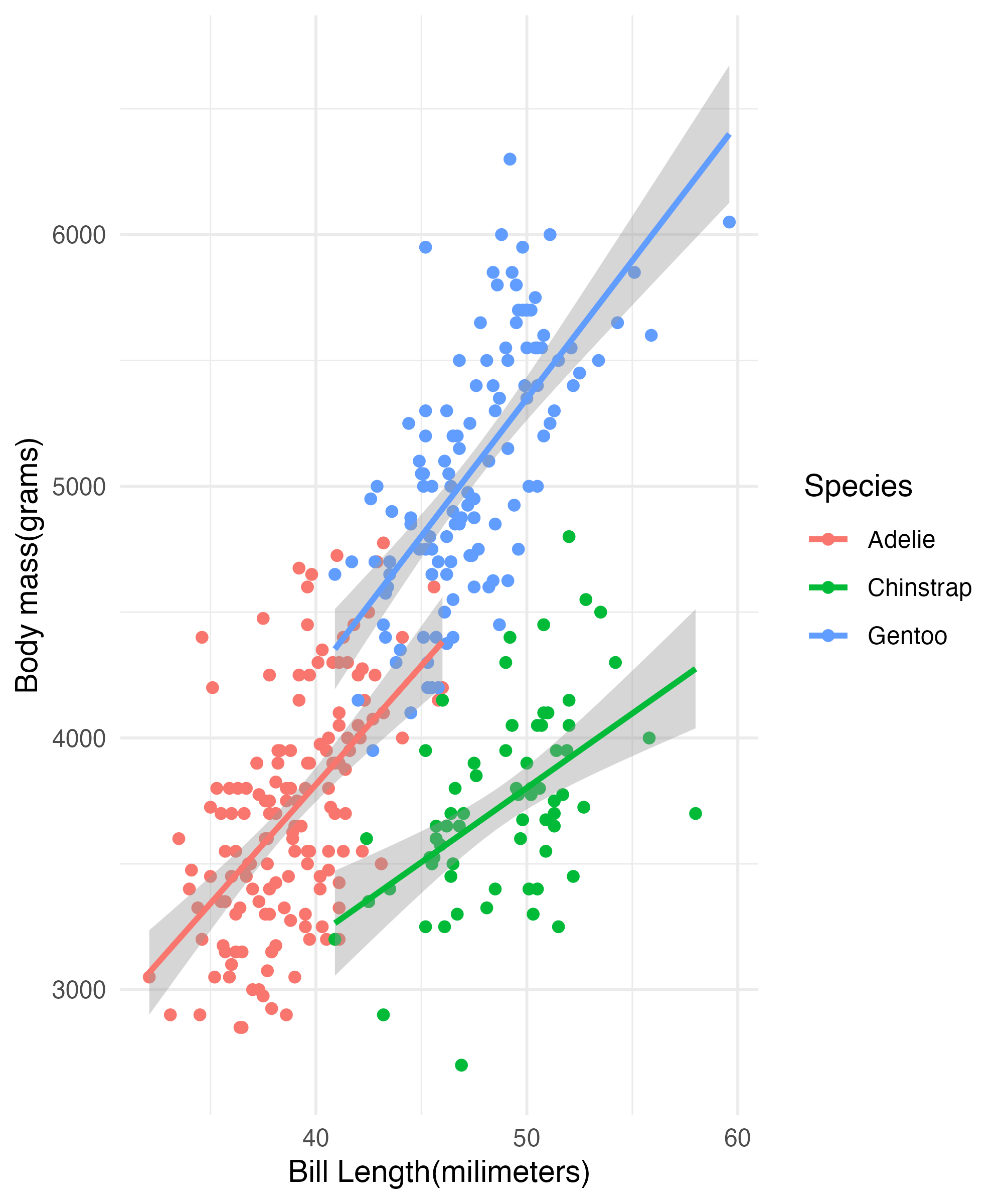
Some Basic Graphs Cont

ggplot(penguins,
   aes(x = bill_depth_mm,
       y = body_mass_g)) +
  geom_point(aes(color = species)) +
  geom_smooth(aes(color = species),
              method = "lm") +
  geom_smooth(method = "lm") + 
  labs(x = "Bill Depth(milimeters)",
        y = "Body mass(grams)") +
  guides(color = guide_legend(title = "Species",
        override.aes = list(fill = NA))) +
  theme_minimal()

Notice that when we plot by subgroup we see evidence of simpson’s pardox

Simpson’s Paradox is a statistical phenomenon where an association between two variables in a population emerges, disappears or reverses when the population is divided into subpopulations. For instance, two variables may be positively associated in a population, but be independent or even negatively associated in all subpopulations

In this case the subgroup differences tell a much different story than the overall population. So that is something that we need to be aware of

Distributions

ggplot(penguins,
  aes(x = flipper_length_mm,
      fill = species)) +
  geom_histogram(alpha = 0.6) +
  labs(x = "Flipper Length(milimeters)") +
  guides(fill = guide_legend(title = "Species")) +
  theme_minimal()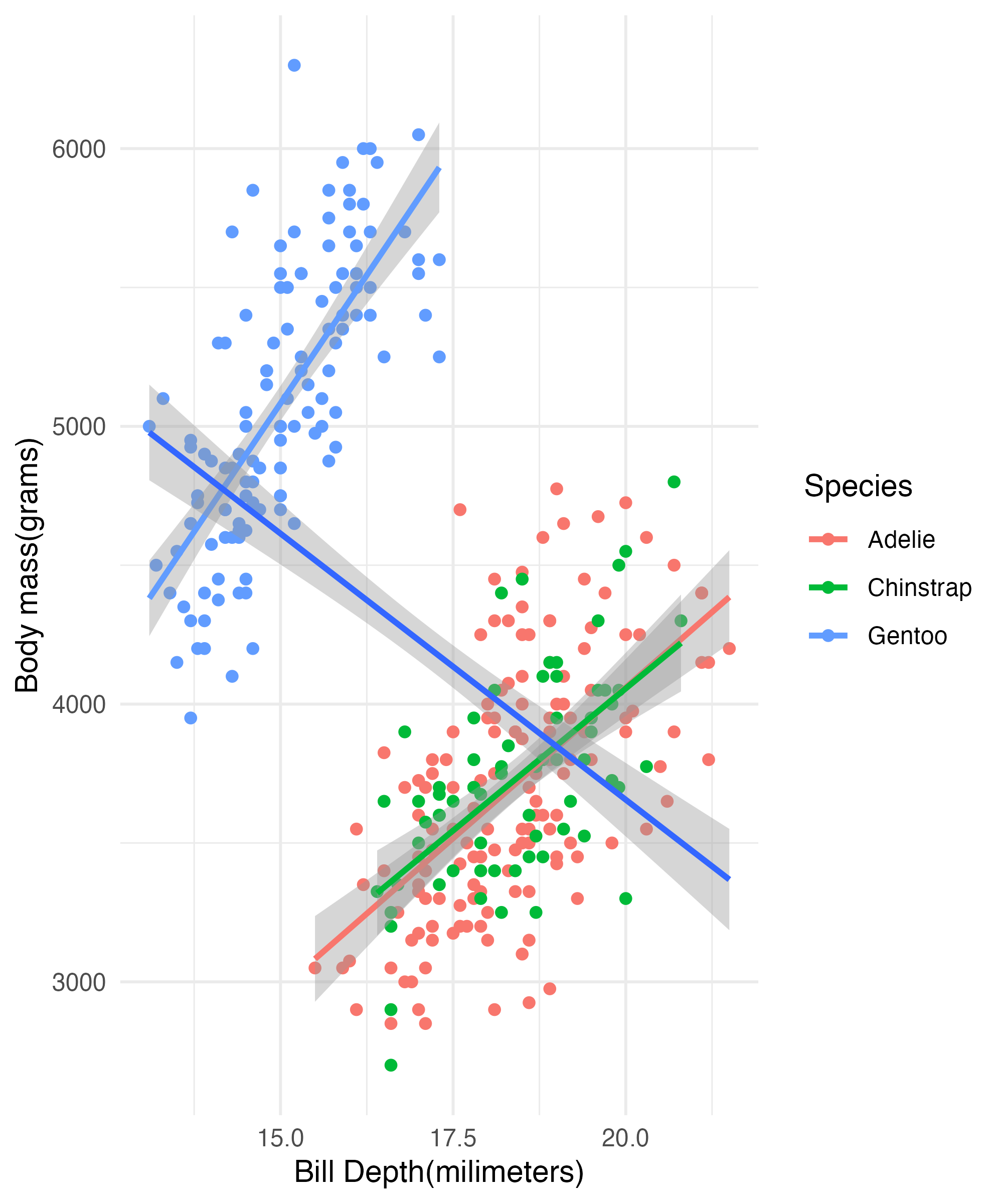

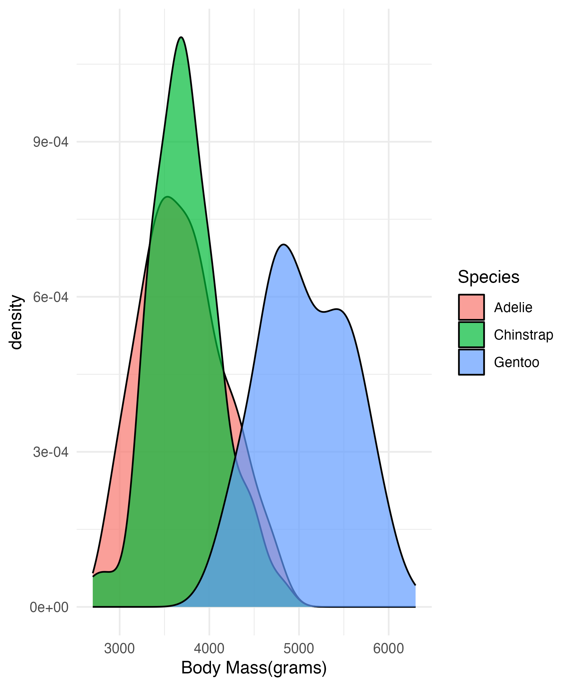
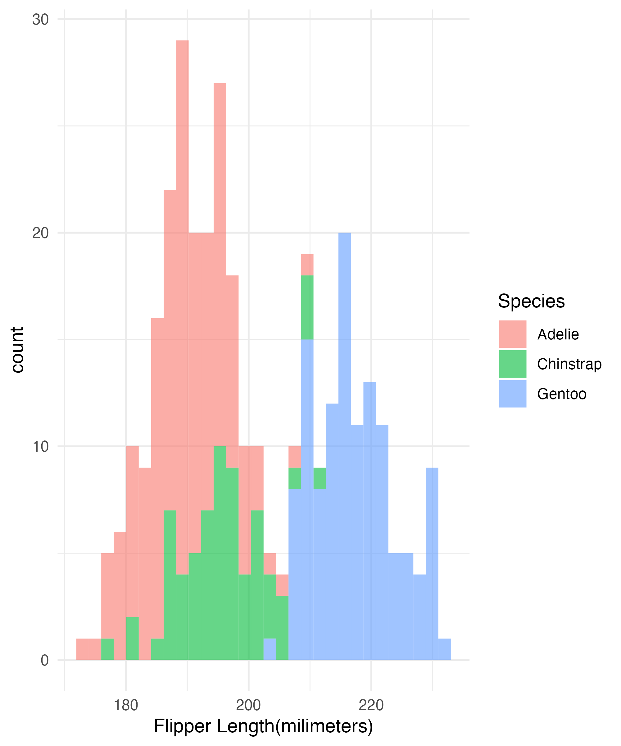
Distributions(cont)

## you can turn off scientific notion 
# using option(scipen = 999)

ggplot(penguins,
  aes(x = body_mass_g,
     fill = species)) +
  geom_density(alpha = 0.7) +
  labs(x = "Body Mass(grams)") +
  guides(fill = guide_legend(title = "Species")) +
  theme_minimal()

User Written Extensions

library(gghalves)
library(MetBrewer)
library(ggdist)

ggplot(penguins,
  aes(x = species,
      y = bill_depth_mm,
     fill = species)) +
  geom_boxplot(
    width = .2, fill = "white",
    size = 1.5, outlier.shape = NA
  ) +
  stat_halfeye(
    adjust = .33,
    width = .67, 
    color = NA,
    position = position_nudge(x = .15)
  ) +
  geom_half_point(
    side = "l", 
    range_scale = .3, 
    alpha = .25, size = 1
  ) +
  scale_fill_met_d(name = "Veronese") +
  labs(x = NULL,
      fill = "Species",
      y = "Bill Depth(millimeters)") +
  coord_flip() +
  theme_minimal()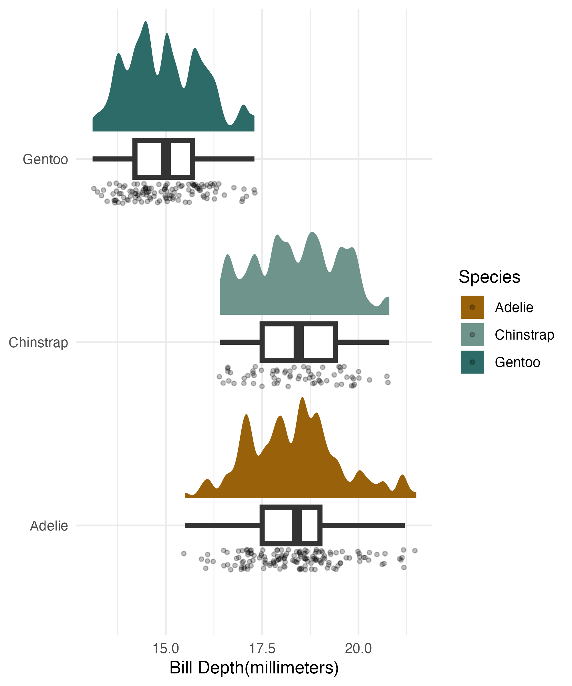

Code and example are from Cédric Scherer’s Beyond the Bar plot talk

Generating Table 1

penguins_df = as.data.frame(penguins) |>
  select(-year)

datasummary(All(penguins_df) ~ Mean + SD + Max + Min + Median + Histogram,
            data = penguins, output = "html",
            title = "Descriptive Statistics") 

Descriptive Statistics

	Mean	SD	Max	Min	Median	Histogram
bill_length_mm	43.92	5.46	59.60	32.10	44.45	▁▅▆▆▆▇▇▂▁
bill_depth_mm	17.15	1.97	21.50	13.10	17.30	▃▄▄▄▇▆▇▅▂▁
flipper_length_mm	200.92	14.06	231.00	172.00	197.00	▂▅▇▄▁▄▄▂▁
body_mass_g	4201.75	801.95	6300.00	2700.00	4050.00	▁▄▇▅▄▄▃▃▂▁

Getting Just A Few Stats

datasummary(body_mass_g + bill_length_mm ~ Mean + SD, data = penguins_df, output = "html")

	Mean	SD
body_mass_g	4201.75	801.95
bill_length_mm	43.92	5.46

Generating a Balance Table

datasummary_balance(~gentoo,
                    data = penguins_t_test)

		FALSE (N=214)		TRUE (N=119)
		Mean	Std. Dev.	Mean	Std. Dev.	Diff. in Means	Std. Error
bill_length_mm		42.0	5.5	47.6	3.1	5.6	0.5
bill_depth_mm		18.4	1.2	15.0	1.0	-3.4	0.1
flipper_length_mm		191.9	7.2	217.2	6.6	25.3	0.8
body_mass_g		3714.7	435.7	5092.4	501.5	1377.7	54.8
year		2008.0	0.8	2008.1	0.8	0.0	0.1
		N	Pct.	N	Pct.
species	Adelie	146	68.2	0	0.0
	Chinstrap	68	31.8	0	0.0
	Gentoo	0	0.0	119	100.0
island	Biscoe	44	20.6	119	100.0
	Dream	123	57.5	0	0.0
	Torgersen	47	22.0	0	0.0
sex	female	107	50.0	58	48.7
	male	107	50.0	61	51.3

Data Analysis in R

Some Basics

estimator(Outcome ~ IV1 + IV2, data = your_data)

• If you want to include all the variables in your data set than you can do that with .

• Remember R can hold lots of datasets so we have to be explicit with where the data is coming from

  • note that we have several different datasets named penguins_blah
  • making sure you have kept track of the using dataset is important

Univariate Regression

peng_naive = lm(body_mass_g ~ bill_length_mm, data = penguins)

peng_naive

Call:
lm(formula = body_mass_g ~ bill_length_mm, data = penguins)

Coefficients:
   (Intercept)  bill_length_mm  
        362.31           87.42  

notice that the output is fairly sparse but in the environment you have a list object in the environment. R creates these as lists because there are tons of things of various classes. So to grab them you can use broom or you can index them.

peng_naive = lm(body_mass_g ~ bill_length_mm, data = penguins)

summary(peng_naive)

Call:
lm(formula = body_mass_g ~ bill_length_mm, data = penguins)

Residuals:
     Min       1Q   Median       3Q      Max 
-1762.08  -446.98    32.59   462.31  1636.86 

Coefficients:
               Estimate Std. Error t value Pr(>|t|)    
(Intercept)     362.307    283.345   1.279    0.202    
bill_length_mm   87.415      6.402  13.654   <2e-16 ***
---
Signif. codes:  0 '***' 0.001 '**' 0.01 '*' 0.05 '.' 0.1 ' ' 1

Residual standard error: 645.4 on 340 degrees of freedom
  (2 observations deleted due to missingness)
Multiple R-squared:  0.3542,    Adjusted R-squared:  0.3523 
F-statistic: 186.4 on 1 and 340 DF,  p-value: < 2.2e-16

This is probably what you are used to seeing if you are coming over from another language

Anova

anova_example = aov(body_mass_g ~ species, data = penguins)

#aov(peng_naive) also works

summary(anova_example)

             Df    Sum Sq  Mean Sq F value Pr(>F)    
species       2 146864214 73432107   343.6 <2e-16 ***
Residuals   339  72443483   213698                   
---
Signif. codes:  0 '***' 0.001 '**' 0.01 '*' 0.05 '.' 0.1 ' ' 1
2 observations deleted due to missingness

TukeyHSD(anova_example)

  Tukey multiple comparisons of means
    95% family-wise confidence level

Fit: aov(formula = body_mass_g ~ species, data = penguins)

$species
                       diff       lwr       upr     p adj
Chinstrap-Adelie   32.42598 -126.5002  191.3522 0.8806666
Gentoo-Adelie    1375.35401 1243.1786 1507.5294 0.0000000
Gentoo-Chinstrap 1342.92802 1178.4810 1507.3750 0.0000000

Here we can see that at least one group is different.

Multiple Regression

peng_adjust = lm(body_mass_g ~  bill_length_mm + flipper_length_mm + species, data = penguins)

summary(peng_adjust)

Call:
lm(formula = body_mass_g ~ bill_length_mm + flipper_length_mm + 
    species, data = penguins)

Residuals:
    Min      1Q  Median      3Q     Max 
-808.83 -230.35  -26.16  223.18 1050.37 

Coefficients:
                   Estimate Std. Error t value Pr(>|t|)    
(Intercept)       -3904.387    529.257  -7.377 1.27e-12 ***
bill_length_mm       61.736      7.126   8.664  < 2e-16 ***
flipper_length_mm    27.429      3.176   8.638 2.34e-16 ***
speciesChinstrap   -748.562     81.534  -9.181  < 2e-16 ***
speciesGentoo        90.435     88.647   1.020    0.308    
---
Signif. codes:  0 '***' 0.001 '**' 0.01 '*' 0.05 '.' 0.1 ' ' 1

Residual standard error: 340.1 on 337 degrees of freedom
  (2 observations deleted due to missingness)
Multiple R-squared:  0.8222,    Adjusted R-squared:  0.8201 
F-statistic: 389.7 on 4 and 337 DF,  p-value: < 2.2e-16

Adding Things in The Formula

peng_adjust_sq = lm(body_mass_g ~  bill_length_mm + flipper_length_mm + I(bill_depth_mm^2) + species, data = penguins)

summary(peng_adjust_sq)

Call:
lm(formula = body_mass_g ~ bill_length_mm + flipper_length_mm + 
    I(bill_depth_mm^2) + species, data = penguins)

Residuals:
    Min      1Q  Median      3Q     Max 
-830.17 -200.27  -20.66  213.11 1049.73 

Coefficients:
                     Estimate Std. Error t value Pr(>|t|)    
(Intercept)        -3215.8543   504.6759  -6.372 6.14e-10 ***
bill_length_mm        43.3825     7.1601   6.059 3.67e-09 ***
flipper_length_mm     20.9168     3.1119   6.721 7.73e-11 ***
I(bill_depth_mm^2)     3.7284     0.5316   7.014 1.28e-11 ***
speciesChinstrap    -535.4478    82.0922  -6.523 2.54e-10 ***
speciesGentoo        847.6827   136.1247   6.227 1.42e-09 ***
---
Signif. codes:  0 '***' 0.001 '**' 0.01 '*' 0.05 '.' 0.1 ' ' 1

Residual standard error: 318.1 on 336 degrees of freedom
  (2 observations deleted due to missingness)
Multiple R-squared:  0.8449,    Adjusted R-squared:  0.8426 
F-statistic: 366.2 on 5 and 336 DF,  p-value: < 2.2e-16

The I is the isolates or inhibit function. R will parse forumulas differently than regualr R code. so ^ has a special meaning in forumla. Which can lead to things that you don’t anticipate. Normally if you wanted to get the sum of two terms you would use the addition symbol to achieve this. But in the formula syntax you are now adding them as terms to the model

from the gaze of R’s formula parsing code. It allows the standard R operators to work as they would if you used them outside of a formula, rather than being treated as special formula operators.

Your Turn

• Estimate a model that looks something like this

lm(flipper_length_mm ~ body_mass_g + other_vars)

• Add any other variables

• what happens if you do this in the equation

lm(flipper_length_mm ~ body_mass_g + log(somevar))

• Bonus: change the factor levels of species so Gentoo is the reference group
  • hint: use fct_relevel or relevel

05:00

penguins = penguins |> mutate(species = fct_relevel(species, “Gentoo”, “Chinstrap”, “Adelie”))

Getting Diagnostic Statistics

Base R

peng_adjust = lm(body_mass_g ~  bill_length_mm + flipper_length_mm + species,
                 data = peng_sans_miss_base)
## remember you need to open the train car door or it will return a listy thing
peng_sans_miss_base$.fitted_vals_brack = peng_adjust[[5]] 

peng_sans_miss_base$.fitted_vals_dollar = peng_adjust$fitted.values

peng_sans_miss_base$.predicted_vals = predict(peng_adjust, interval = "prediction")

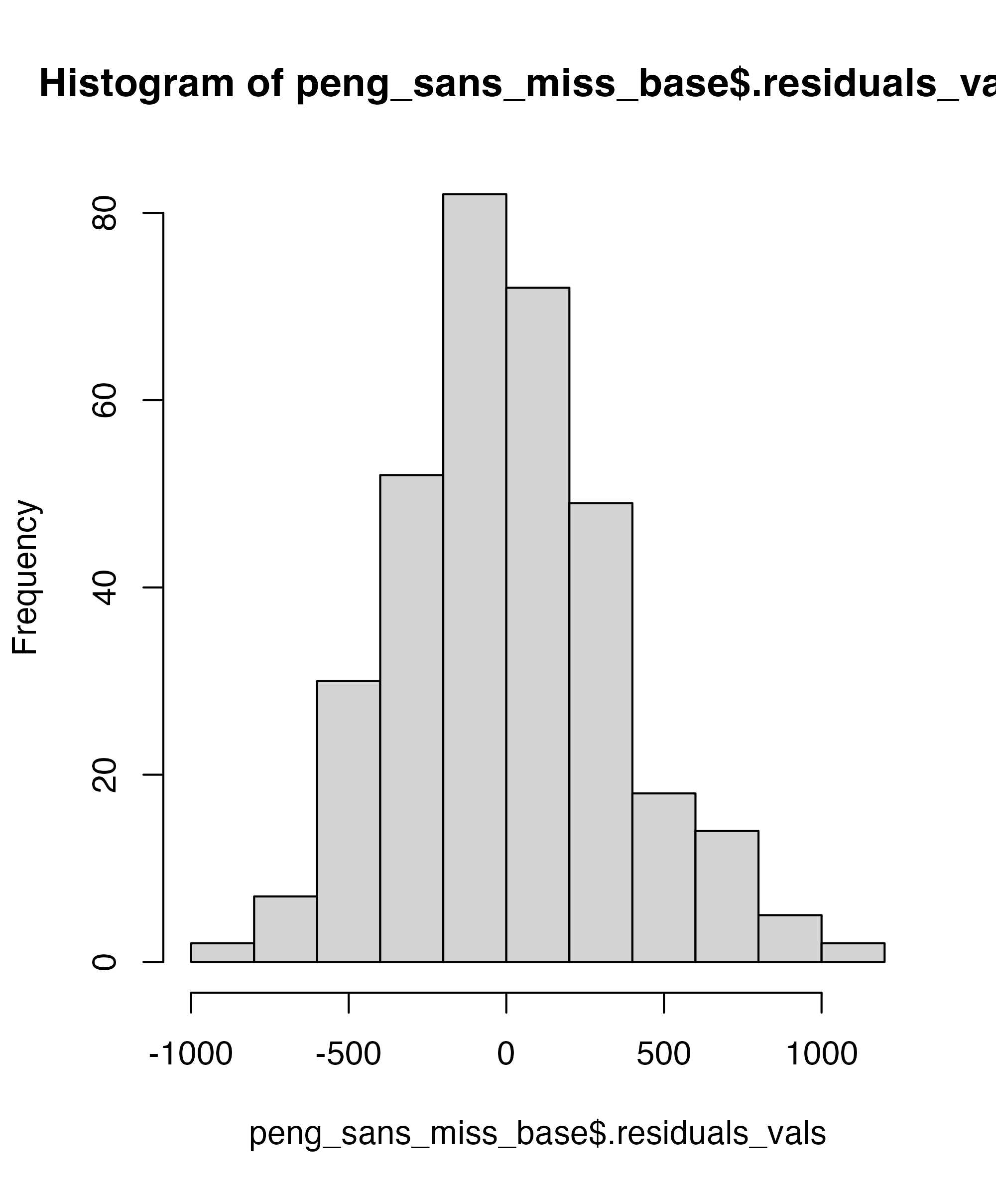
peng_sans_miss_base$.residuals_vals = peng_adjust$residuals

peng_sans_miss_base$.studentized_resids = rstudent(peng_adjust)

peng_sans_miss_base$.cooks_distance = cooks.distance(peng_adjust)

Tidyverse

peng_adjust = lm(body_mass_g ~  bill_length_mm + flipper_length_mm + species,
   data = peng_sans_miss_tidy) 
peng_diag_tidy = augment(peng_adjust,
                         data = peng_sans_miss_tidy)

As good data analysts we should always check that our assumptions are met. One really good test is to just plot our fitted values against our residuals. So lets go ahead and grab them. In base you just index them via the dollar sign or brackets. In the tidyverse can get them via broom augment. They will be returned with the name of the thing you want starting with a dot.

The reason is that the team behind broom did not want to override existing stuff

I just dropped the missing values to make my life easier

Plotting

Base

plot(peng_sans_miss_base$.fitted_vals_dollar,
     peng_sans_miss_base$.residuals_vals,
     col = peng_sans_miss_base$species)
abline(lm(peng_sans_miss_base$.residuals_vals ~ peng_sans_miss_base$.fitted_vals_dollar))

Tidyverse

ggplot(peng_diag_tidy, aes(x = .fitted,
                           y = .resid)) +
  geom_point(aes(color = species)) +
  geom_smooth(method = "lm") +
  theme_minimal()

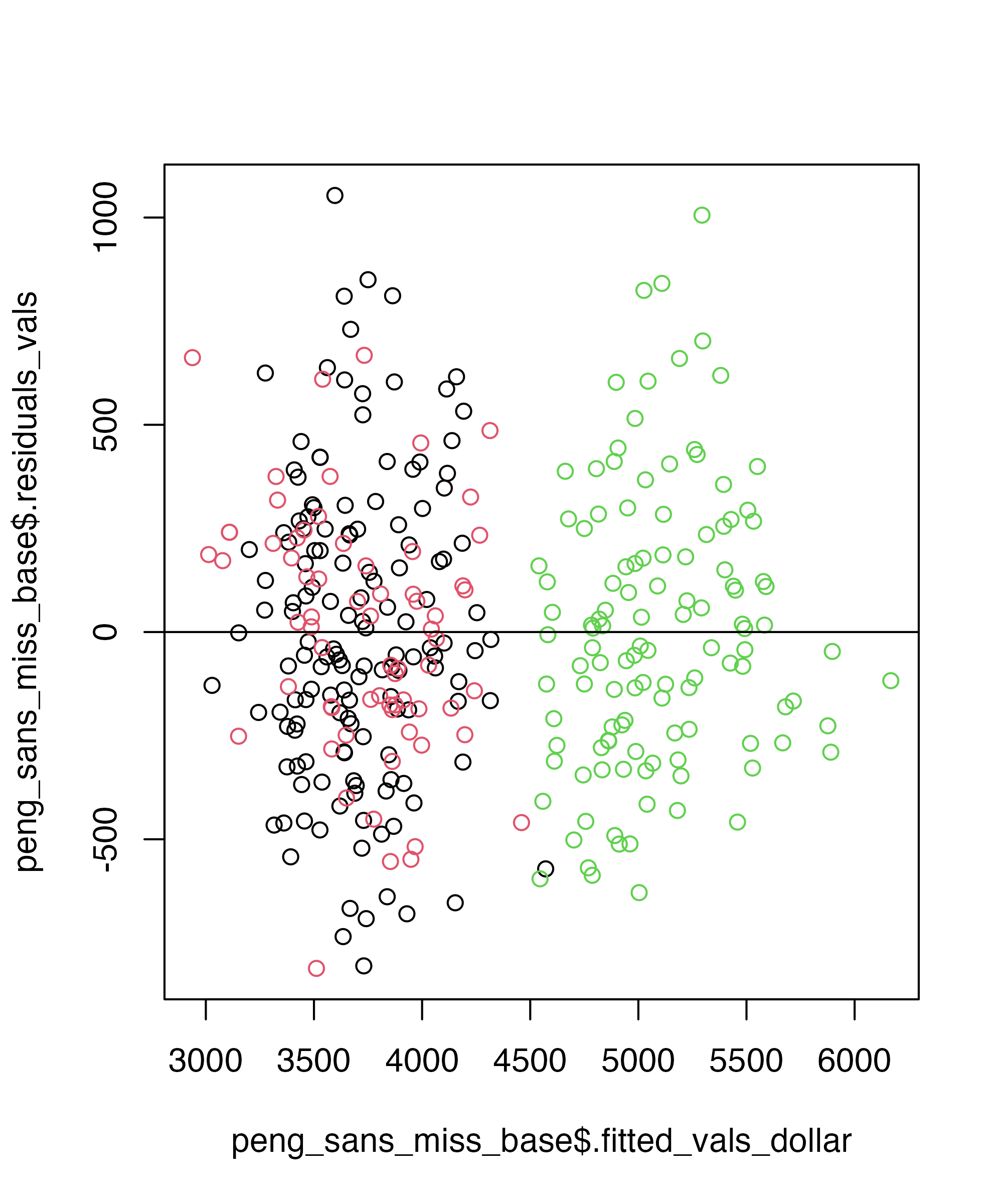
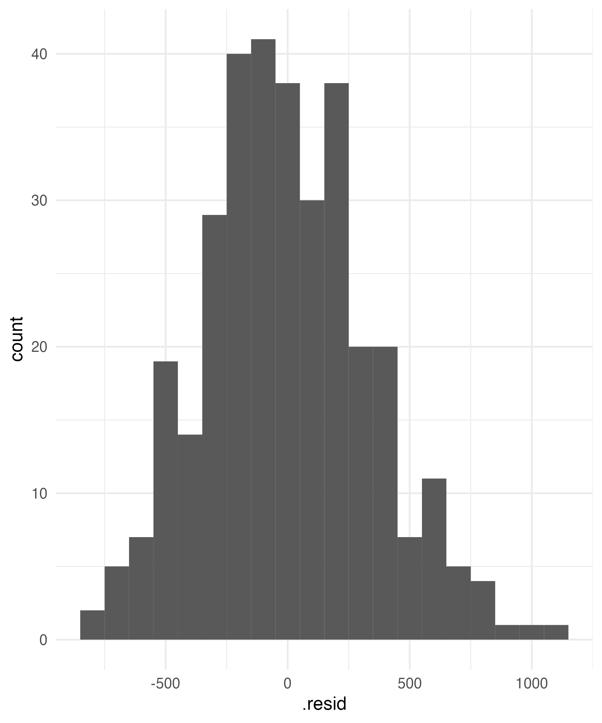
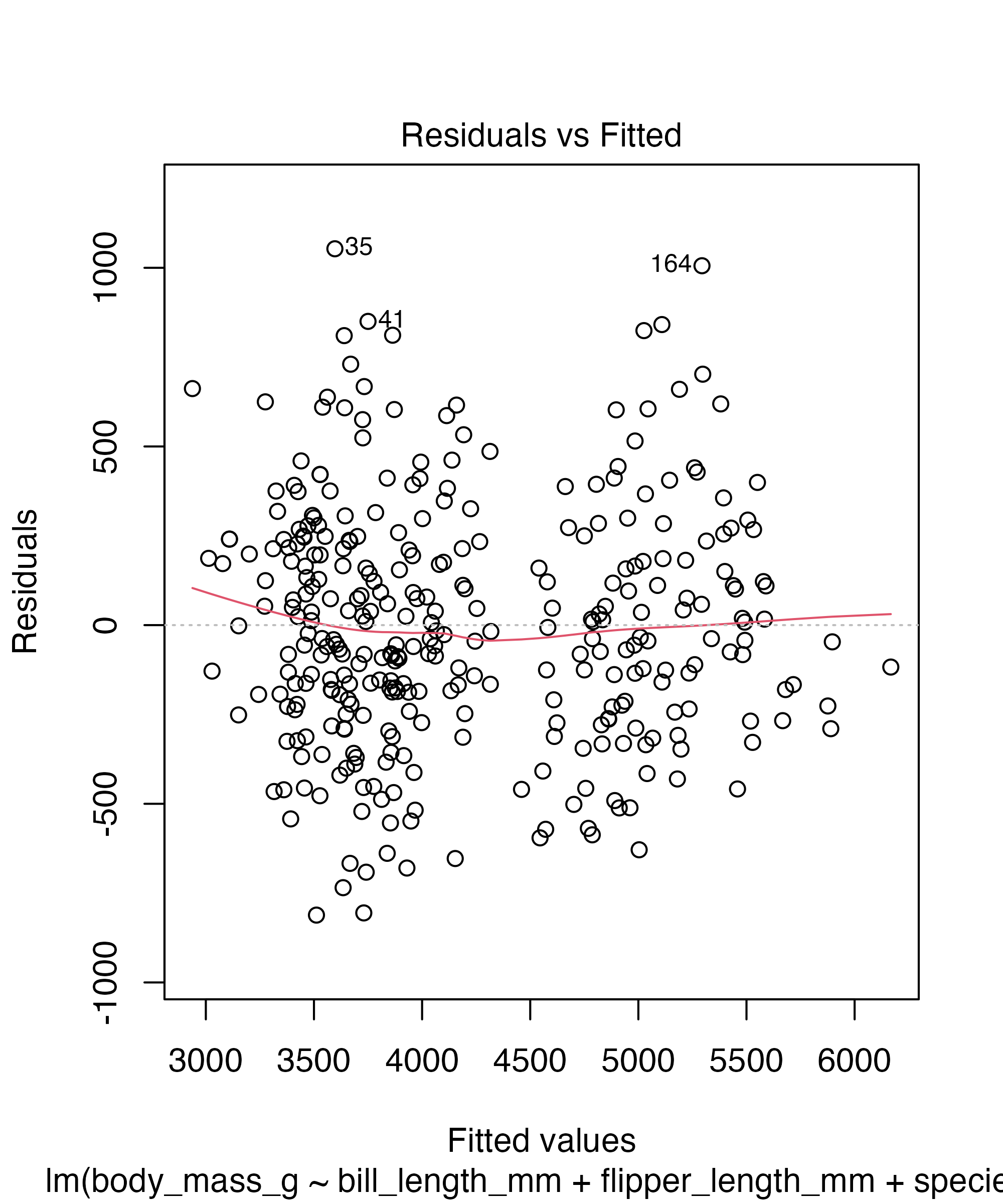
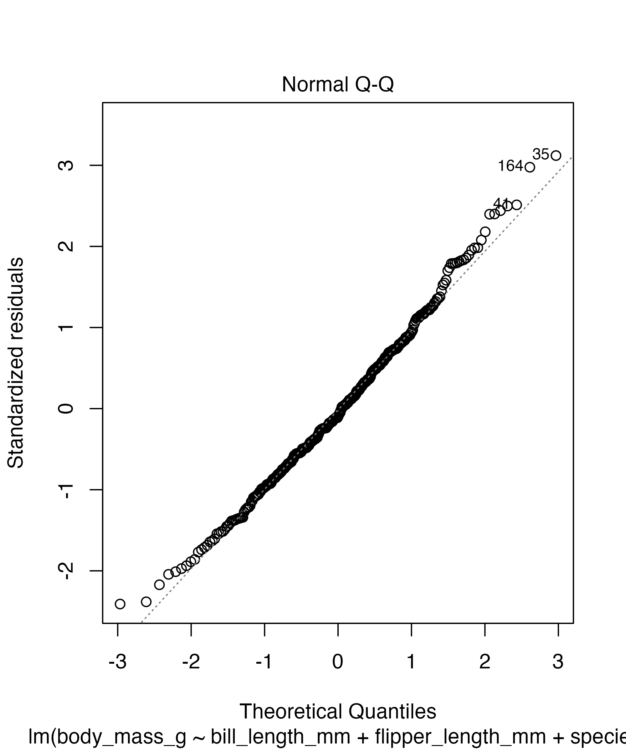
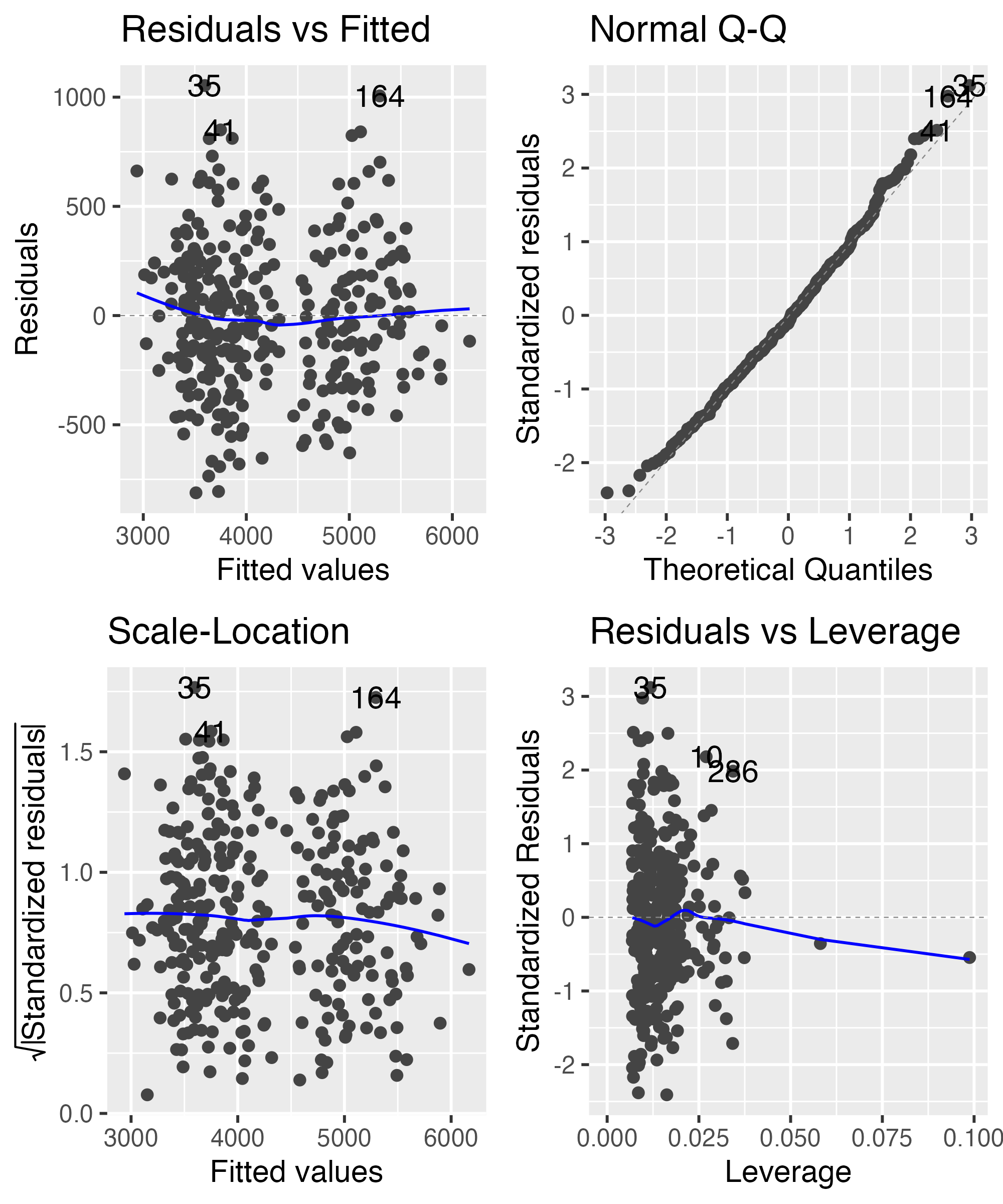
Checking for Normality

hist(peng_sans_miss_base$.residuals_vals)
ggplot(peng_diag_tidy, aes(x = .resid)) +
  geom_histogram(binwidth = 100) +
  theme_minimal()

Base R diagnostic plots

par(mfrow = c(2, 2))
plot(peng_adjust)

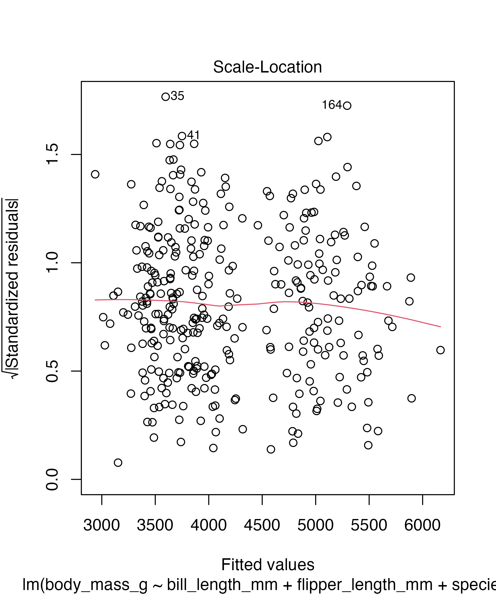
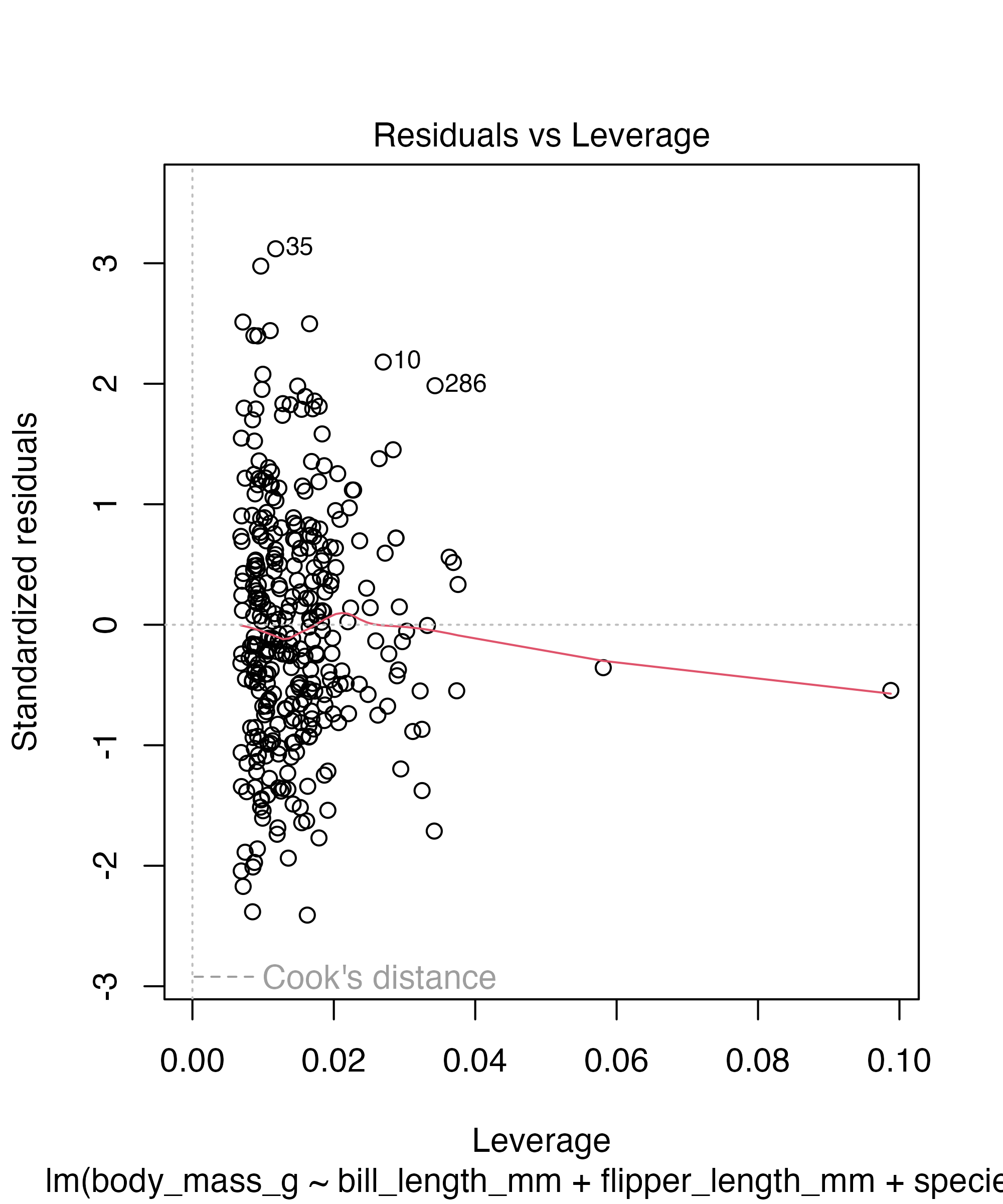
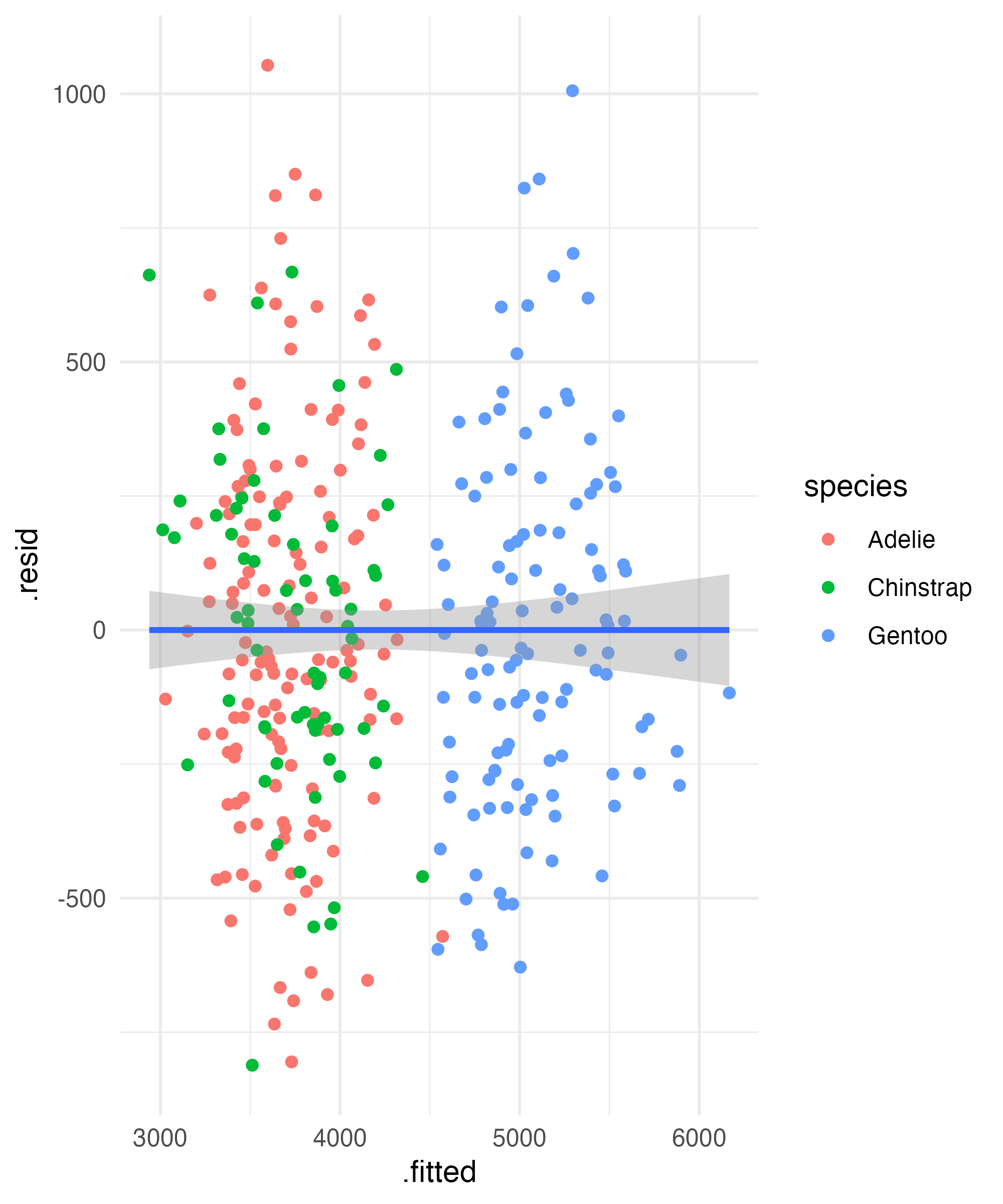
ggplot2 extension for same thing

autoplot(peng_adjust)

Tests

bptest(peng_adjust)

statistic	p.value	parameter	method
3.678191	0.4513059	4	studentized Breusch-Pagan test

bgtest(peng_adjust)

statistic	p.value	parameter	method
8.776406	0.0030515	1	Breusch-Godfrey test for serial correlation of order up to 1

null for Breusch Pagan there is no hetrosckedasticity

fail to reject the null hypothesis. This means that there is no heterosckedasticity. Thats awesome

Null for Breusch Godfrey is there is no serial correlation of order up to 1

We can reject the null hypothesis meaning that there is some autocorrelation in our data.

Okay it looks like something we have violated some of our assumptions

Your Turn(optional)

• Get the fitted and and residuals from your multiple regression

• Are the regression assumptions met?

• Look through the lmtest documentation to see what other tests are available.

Fixing Our Standard Errors

• We can do this “on the fly” in R

• There are ways to do this in the model formula with various packages

  • But it is better to do this “on the fly”

Adjusting Our Standard Errors for Real This time

coeftest(peng_adjust, vcov= vcovHC)

t test of coefficients:

                    Estimate Std. Error t value  Pr(>|t|)    
(Intercept)       -3864.0732   507.3100 -7.6168 2.807e-13 ***
bill_length_mm       60.1173     6.5195  9.2212 < 2.2e-16 ***
flipper_length_mm    27.5443     3.0951  8.8993 < 2.2e-16 ***
speciesChinstrap   -732.4167    76.3112 -9.5978 < 2.2e-16 ***
speciesGentoo       113.2542    89.2584  1.2688    0.2054    
---
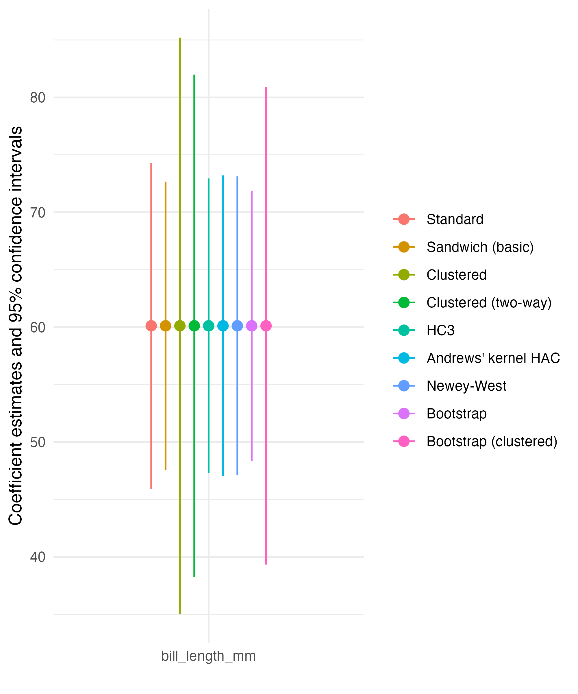
Signif. codes:  0 '***' 0.001 '**' 0.01 '*' 0.05 '.' 0.1 ' ' 1

Using sandwich we can adjust our standard errors like this

A Whole Host of Standard Errors

vc <- list(
  "Standard"              = vcov(peng_adjust),
  "Sandwich (basic)"      = sandwich(peng_adjust),
  "Clustered"             = vcovCL(peng_adjust, cluster = ~ species),
  "Clustered (two-way)"   = vcovCL(peng_adjust, cluster = ~ species + year),
  "HC3"                   = vcovHC(peng_adjust),
  "Andrews' kernel HAC"   = kernHAC(peng_adjust),
  "Newey-West"            = NeweyWest(peng_adjust),
  "Bootstrap"             = vcovBS(peng_adjust),
  "Bootstrap (clustered)" = vcovBS(peng_adjust, cluster = ~ species)
)

Base

adjusted_models = lapply(vc, function(x) coeftest(peng_adjust, vcov = x))

Tidy

map_version = map(vc, ~coeftest(peng_adjust, vcov = .x))

We can feed a huge list of standard errors fairly quickly it this took virtually no time. Instead of going back and adjusting a huge set of models as would be the case in other softwares where you specify standard error fixes in the model here you can simply specify it once and forget it.

What does it look like?

Making Table 2

• Model Summary is my favorite table making package
  • if you run modelsummary::supported_models() you will see it fits most needs
  • Once awesome feature is adjusting your standard errors while making the table!

se_info = tibble(term = "Standard errors","iid", "robust", "bootstrap", "stata", "clustered by sex")
modelsummary(peng_adjust,
             stars = TRUE,
             coef_omit = "(Intercept)|flipper_length_mm|.*species",
             add_rows = se_info,
             vcov =  list("iid", "robust", "bootstrap", "stata", cluster = ~ sex ),
             gof_map = c("nobs", "r.squared"))

The Results

	(1)	(2)	(3)	(4)	(5)
bill_length_mm	60.117***	60.117***	60.117***	60.117***	60.117***
	(7.207)	(6.519)	(7.063)	(6.429)	(1.591)
Num.Obs.	333	333	333	333	333
R2	0.824	0.824	0.824	0.824	0.824
Standard errors	iid	robust	bootstrap	stata	clustered by sex
+ p < 0.1, * p < 0.05, ** p < 0.01, *** p < 0.001

Saving Tables

• If you do not work in Quarto like me this is how you save tables to include in a manuscript
  • One tip for word users. Save it as an html and open the html file in word and copy and paste

modelsummary(models, output = "table.docx")
modelsummary(models, output = "table.html")
modelsummary(models, output = "table.tex")
modelsummary(models, output = "table.md")
modelsummary(models, output = "table.txt")
modelsummary(models, output = "table.png")

Handling Missing Data

• The default in R is to use listwise deletion

• This requires some assumptions about why the data is missing

• Sometimes we may need to impute data for missing observations

mods <- list()

pengs_impute_mice = mice::mice(penguins, m = 5, printFlag = FALSE)

pengs_amelia = Amelia::amelia(as.data.frame(penguins), m = 5, p2s = 0,
                               idvars = c("species", "island", "sex"))$imputations

mods[['List Wise Deletion']] = lm(body_mass_g ~  bill_length_mm + flipper_length_mm + species,
   data = penguins)

mods[['Mice']] = with(pengs_impute_mice,lm(body_mass_g ~ bill_length_mm + flipper_length_mm + species))
mods[['Amelia']] = lapply(pengs_amelia, \(x) lm(body_mass_g ~  bill_length_mm + flipper_length_mm + species, data = x))

mods[['Mice']] <- mice::pool(mods[['Mice']])

mods[['Amelia']] <- mice::pool(mods[['Amelia']])

Missing data is a fact of life when you work with real data. So we have to deal with it. Just letting R drop it makes very strong assumptions about why the data is missing. Often times we may want to

Lets see it in a table

	List Wise Deletion	Mice	Amelia
(Intercept)	−3904.387	−3888.376	−4029.226
	(529.257)	(528.070)	(579.288)
bill_length_mm	61.736	61.436	60.274
	(7.126)	(7.108)	(7.677)
flipper_length_mm	27.429	27.410	28.380
	(3.176)	(3.170)	(3.287)
speciesChinstrap	−748.562	−746.236	−738.515
	(81.534)	(81.265)	(89.494)
speciesGentoo	90.435	92.497	77.150
	(88.647)	(88.331)	(100.817)
R2	0.822	0.823	0.820
Num.Obs.	342	344	344
RMSE	337.62

Interactions

• To include a multiplicative term we can use *, :
  • These differ slightly
• The constitutive terms will appear automatically with *

pengs_interact_stand = lm(body_mass_g ~ bill_length_mm * sex + species + flipper_length_mm,
                           data = peng_sans_miss_tidy)

pengs_interact_col = lm(body_mass_g ~ bill_length_mm * sex + sex + species + bill_length_mm + flipper_length_mm ,
                           data = peng_sans_miss_tidy)

summary(pengs_interact_stand)

Call:
lm(formula = body_mass_g ~ bill_length_mm * sex + species + flipper_length_mm, 
    data = peng_sans_miss_tidy)

Residuals:
    Min      1Q  Median      3Q     Max 
-722.25 -189.89   -5.58  188.97  897.79 

Coefficients:
                        Estimate Std. Error t value Pr(>|t|)    
(Intercept)            -1279.184    601.073  -2.128 0.034073 *  
bill_length_mm            28.695      7.980   3.596 0.000374 ***
sexmale                 1004.946    279.166   3.600 0.000368 ***
speciesChinstrap        -302.268     81.331  -3.716 0.000238 ***
speciesGentoo            670.469     95.795   6.999 1.47e-11 ***
flipper_length_mm         19.052      2.954   6.449 4.06e-10 ***
bill_length_mm:sexmale   -12.525      6.403  -1.956 0.051324 .  
---
Signif. codes:  0 '***' 0.001 '**' 0.01 '*' 0.05 '.' 0.1 ' ' 1

Residual standard error: 290.7 on 326 degrees of freedom
Multiple R-squared:  0.872, Adjusted R-squared:  0.8697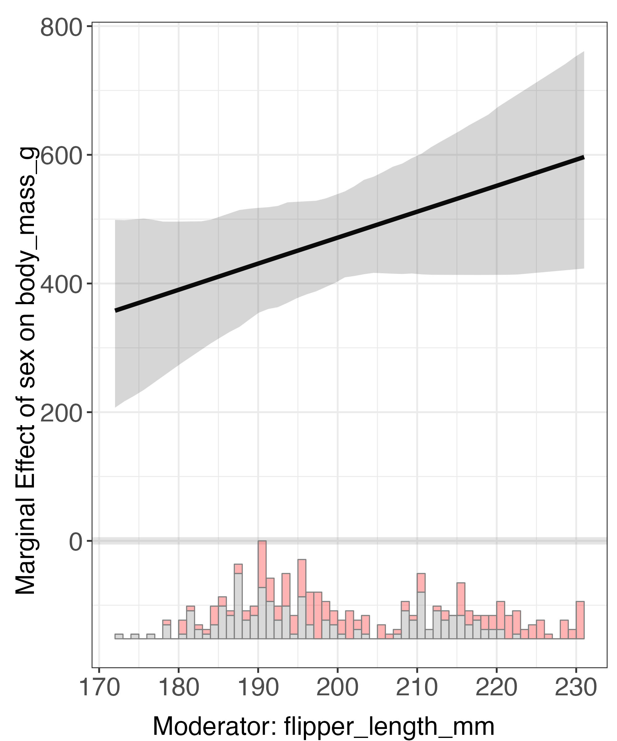 
F-statistic: 370.2 on 6 and 326 DF,  p-value: < 2.2e-16

The nice part about R is that you can include interactions in a few different ways. One thing is that R will include the constuitive terms for you. The slash will sort of trick R into including the full marginal effects for you.

Getting Marginal Effects for Interactions

library(marginaleffects)
pengs_interact_effect = lm(body_mass_g ~ bill_length_mm  + flipper_length_mm * sex + species, data = peng_sans_miss_tidy)

plot_comparisons(
  pengs_interact_effect,
  condition =  "flipper_length_mm",
  variables = "sex") +
  labs(x = "Bill Length(mm)", y = "Unit Level Conditional Estimates") +
  theme_minimal()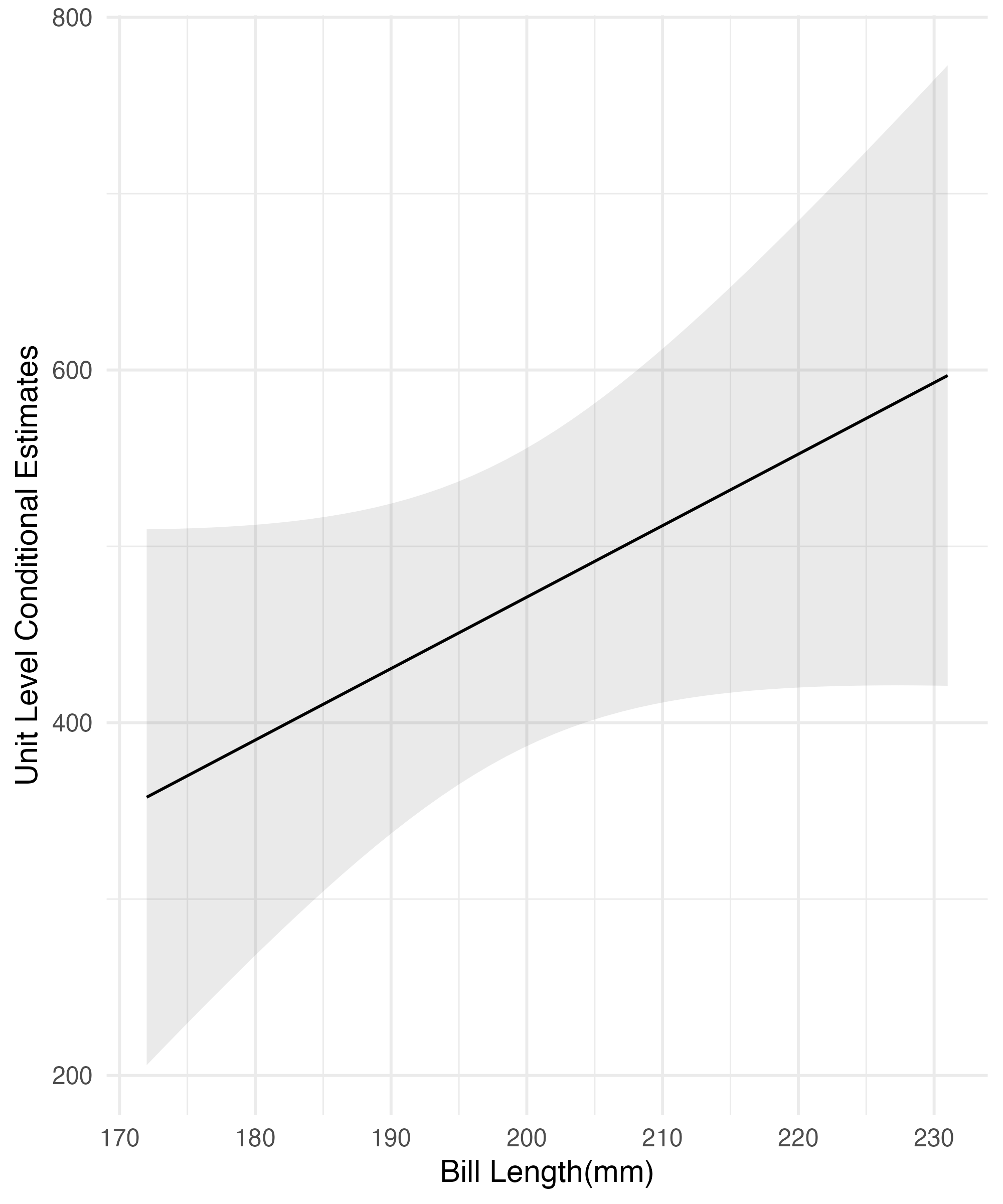

We may be interested in what happens when we shift the values of our continous variable. One awesome way to do this is through our marginal effects package. In this case we can look at the effect as bill_length_mm and the conditonal contrasts. plot cco plots the contrasts (y-axis) against values of predictor(s) variable(s) (x-axis and colors).

essentially what happens when we have an increase of some value

So in this case this is just showing the effect when penguins take on the value of male and flipper length in increases by x amount mm

Interflex

library(interflex)

peng_interflex = as.data.frame(peng_sans_miss_tidy)


interflex(Y = "body_mass_g",
          D = "sex",
          X = "flipper_length_mm",
          Z = c("bill_length_mm", "species"),
         estimator = "kernel",
         data = peng_interflex,
         theme.bw = TRUE,
         parallel = FALSE) # recommend that you set this to true

Interflex is also a package that I would be remiss not to bring attention to. It is by a group of political scientists. This implements some tests to ensure that there is a linear interaction effects and whether there is common support. Basically if you start to plug in values your self across the full range of flipper lenghh you may be calculating effects where there is not a ton of data making those estimates super fragile. I would probably opt for interflex in this case but I think that is just a discipline specific thing

The kernal estimator is what they reccommend. It is more flexible because we are not imposing a strong parametric form of the relationship. It is also nice because we include any confounders. So it looks like when we increase our flipper length in mm to about 190 mm the body mass of the penguins increase to about 400 g

Tables with multiple models

modelsummary(list(peng_naive, peng_adjust, pengs_interact_stand),
             stars = TRUE,
             gof_omit = ".*", ## omitting all goodness of fit for space
             coef_map = c("bill_length_mm" = "Bill Length(mm)",
                          "flipper_length_mm" = "Flipper Length(mm)",
                          "bill_length_mm:sexmale" = "Bill Length(mm) x Male Penguin"),
             vcov = "robust",
             note = "Robust Standard errors in Parenthsis")

	(1)	(2)	(3)
Bill Length(mm)	87.415***	60.117***	28.695***
	(6.898)	(6.519)	(6.817)
Flipper Length(mm)		27.544***	19.052***
		(3.095)	(2.910)
Bill Length(mm) x Male Penguin			−12.525*
			(6.207)
+ p < 0.1, * p < 0.05, ** p < 0.01, *** p < 0.001
Robust Standard errors in Parenthsis

Fancy Tables

• Often times we have multiple dv’s

• A popular strategy in Pols and Econ is to make a table with two panels

  • Where outcome 1 is in one panel and outcome two is in the bottom panel

gm <- c("r.squared", "nobs", "rmse")

panels <- list(
  list(
    lm(body_mass_g ~ bill_length_mm + species, data = peng_sans_miss_tidy),
    lm(body_mass_g ~ bill_length_mm, data = peng_sans_miss_tidy)
  ),
  list(
    lm(flipper_length_mm ~ species + bill_length_mm, data = peng_sans_miss_tidy),
    lm(flipper_length_mm ~ species + bill_length_mm + bill_depth_mm, data = peng_sans_miss_tidy)
  )
)

modelsummary(
  panels,
  shape = "rbind",
  gof_map = gm)

Output

	(1)	(2)
Panel A
(Intercept)	200.453	388.845
	(271.646)	(289.817)
bill_length_mm	90.298	86.792
	(6.951)	(6.538)
speciesChinstrap	-876.942
	(88.744)
speciesGentoo	596.702
	(76.429)
R2	0.785	0.347
RMSE	372.93	649.48
Panel B
(Intercept)	147.563	127.187
	(4.223)	(5.250)
speciesChinstrap	-5.247	-1.519
	(1.380)	(1.450)
speciesGentoo	17.552	27.394
	(1.188)	(1.987)
bill_length_mm	1.096	0.709
	(0.108)	(0.121)
bill_depth_mm		1.929
		(0.320)
R2	0.828	0.845
RMSE	5.80	5.50
Num.Obs.	333	333

Fixed Effects

• Mega popular estimation strategy in Econ and Political Science

library(plm)
library(vdemdata)

vdem_feols = feols(v2x_polyarchy ~ v2x_gender + v2x_corr | year + country_id, data = vdem)

vdem_stand = lm(v2x_polyarchy ~ v2x_gender + v2x_corr + factor(year) + factor(country_id), data = vdem)

vdem_plm = plm(v2x_polyarchy ~ v2x_gender + v2x_corr + factor(year), 
  data = vdem,
  index = c("country_id"),
  model = "within")

There are more than a few ways to get a fixed effects regression in R my prefered way is using fixest. Because a species and island fixed effect would be a bit ridicoulous we can use star wars to demonstrate our point a bit. Feols does this in a really intuitive way. All your fixed effectgs are behi

To sort of get on with the rest of the workshop I will not spend to much time on this. But it is stupid fast and lets you do a whole lot. It does not have random effects tho. PLM is really useful for lots of other common panel estimators. But fixest is still the winner when it comes to] fixed effects models.

Performance

• Vdem has 202 country ids and 233 years
  • Lets time them to see

# A tibble: 3 × 2
  expr       `Mean Time in Seconds`
  <fct>                       <dbl>
1 vdem_feols                0.00182
2 vdem_stand                0.479  
3 vdem_plm                  0.367  

Your Turn

• Create and indicator variable for the chinstrap penguin species

• Add an interaction term with bill depth in a regression

• create a table with modelsummary with all your models

05:00

Generating Predictions

set.seed(1994)

penguins_prediction = mutate(penguins, id = row_number()) |> 
drop_na()

peng_train = penguins_prediction |> 
  sample_frac(0.7) # sample 70% of the dataset 

peng_test = anti_join(penguins_prediction, peng_train, by = "id")

peng_test$data_set = "Test" # add an indicator for what data set we have

penguins_training_model = lm(body_mass_g ~ bill_length_mm, data = peng_train)

penguins_train_plot = augment(penguins_training_model, 
                      interval = "prediction") |>
                      select(.fitted, .lower, .upper, body_mass_g, bill_length_mm) |>
                      mutate(data_set = "train")

# alterntively this works
# predict(penguins_train_plot, newdata = peng_test)

peng_predict_test = augment(penguins_training_model,
                           interval = "prediction",
                           newdata = peng_test) |> 
 select(.fitted, .lower, .upper,  body_mass_g, bill_length_mm, data_set) |>
 bind_rows(penguins_train_plot)

It involves randomly dividing the available set of observations into two parts, a training set and a validation set or hold-out set. The model is fit on the training set, and the fitted model is used to predict the responses for the observations in the validation set. The resulting validation set error rate — typically assessed using MSE in the case of a quantitative response—provides an estimate of the test error rate.

generating predictions from a model is really useful for lots of places. So being able to do it from a very simple model is important. The general principles apply in a variety of cases. You may need the predicted probabiilities for propensity score matching or inverse probability weighting

Visual Inspection

ggplot(peng_predict_test,
  aes(x = bill_length_mm,
    y = body_mass_g,
   color = data_set,
    fill = data_set)) +
  geom_point(alpha = 0.7) +
  geom_line(aes(y = .fitted)) +
  geom_ribbon(aes(ymin = .lower,
             ymax = .upper),
               alpha = 0.3,
               col = NA) +
  scale_color_discrete(name = "Training sample?",
                       aesthetics = c("color",
                                      "fill")) +
  theme_minimal()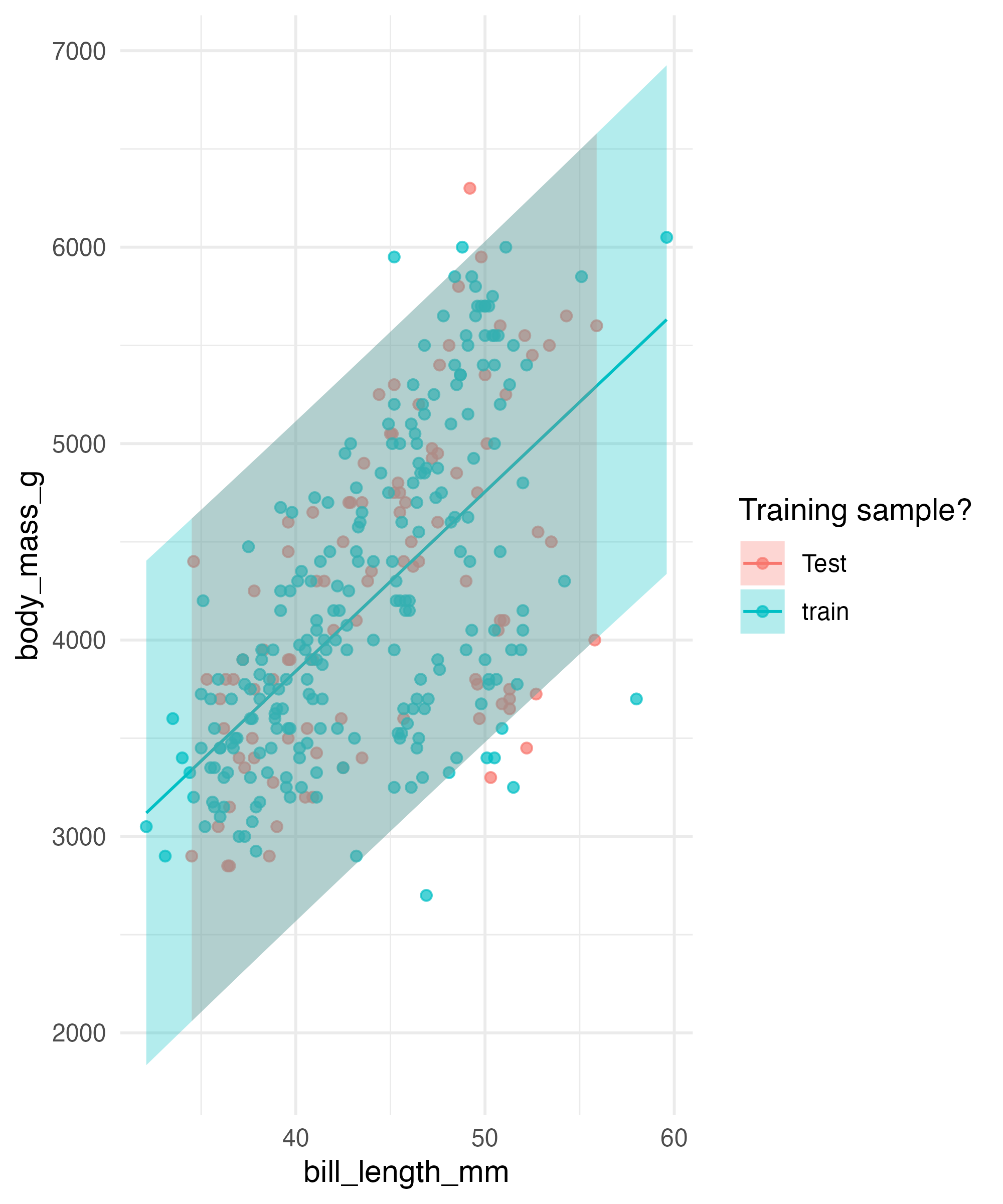

Maximum Likelihood Estimation
Machine Learning

• R comes with a whole host of maximum likelihood estimators(MLE)

  • As well as user written packages

• You will also probably want to load marginaleffects to get marginal effects of your model

  • Remember the coefficients of a MLE model are not directly interpretable

• emmeans is also a solid package for getting marginal effects

• Note: They do differ on what they can do and how they generate marginal effects

  • Andrew Heiss has a nice summary of this at the bottom of this blog post

The data we are using

penguins_glm = penguins |> 
  drop_na() |> 
  mutate(big_penguin = ifelse(body_mass_g > median(body_mass_g), 1,0),
         big_penguin_logic = ifelse(body_mass_g > median(body_mass_g), TRUE, FALSE),
         female = ifelse(sex == "female", TRUE, FALSE))

Lets See What this looks like

ggplot(penguins_glm,
    aes(x = bill_length_mm,
       y = big_penguin)) +
  stat_dots(aes(side = ifelse(big_penguin == 0,
       "top",
       "bottom")),
       scale = 1/3) +
  geom_smooth(method = "glm",
  method.args = list(family = binomial(link = "logit"))) +
  theme_minimal()

Our Model

base_model = glm(big_penguin ~ bill_length_mm + flipper_length_mm + species + female,
                 data = penguins_glm,
                 family = binomial(link = "logit"))

summary(base_model)

Call:
glm(formula = big_penguin ~ bill_length_mm + flipper_length_mm + 
    species + female, family = binomial(link = "logit"), data = penguins_glm)

Deviance Residuals: 
    Min       1Q   Median       3Q      Max  
-2.5554  -0.1754  -0.0458   0.1525   3.3236  

Coefficients:
                   Estimate Std. Error z value Pr(>|z|)    
(Intercept)       -28.21658    7.65713  -3.685 0.000229 ***
bill_length_mm      0.16149    0.10149   1.591 0.111593    
flipper_length_mm   0.11095    0.03734   2.971 0.002966 ** 
speciesChinstrap   -3.06047    1.16962  -2.617 0.008880 ** 
speciesGentoo       4.77533    1.71546   2.784 0.005374 ** 
femaleTRUE         -3.30482    1.07008  -3.088 0.002013 ** 
---
Signif. codes:  0 '***' 0.001 '**' 0.01 '*' 0.05 '.' 0.1 ' ' 1

(Dispersion parameter for binomial family taken to be 1)

    Null deviance: 461.27  on 332  degrees of freedom
Residual deviance: 147.40  on 327  degrees of freedom
AIC: 159.4

Number of Fisher Scoring iterations: 8

For fitting glm’s in R you use the glm fucntion. The built in function supports like a handful of glm’s. So you have probit, logit, poisson, binomial and quasi poisson. There are various package to get like a negative binomial model. I know the bayesians love themselves an ordered betareg.

Getting Interpretable Quantities

# get odds ratio

odds_ration = exp(coef(base_model))

 marginal_effect = base_model |> 
  slopes()  |> 
  tidy()

ggplot(data = filter(marginal_effect,
       !term == "species"),
       aes(x = estimate,
           y = str_to_title(term))) +
  geom_pointrange(aes(xmin = conf.low,
                     xmax = conf.high)) +
  geom_vline(xintercept = 0) +
  labs(y = NULL,
       x = "Average Marginal Effect") +
  theme_minimal()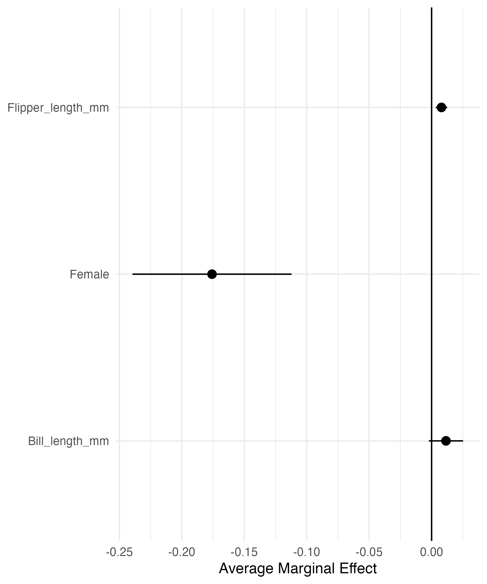

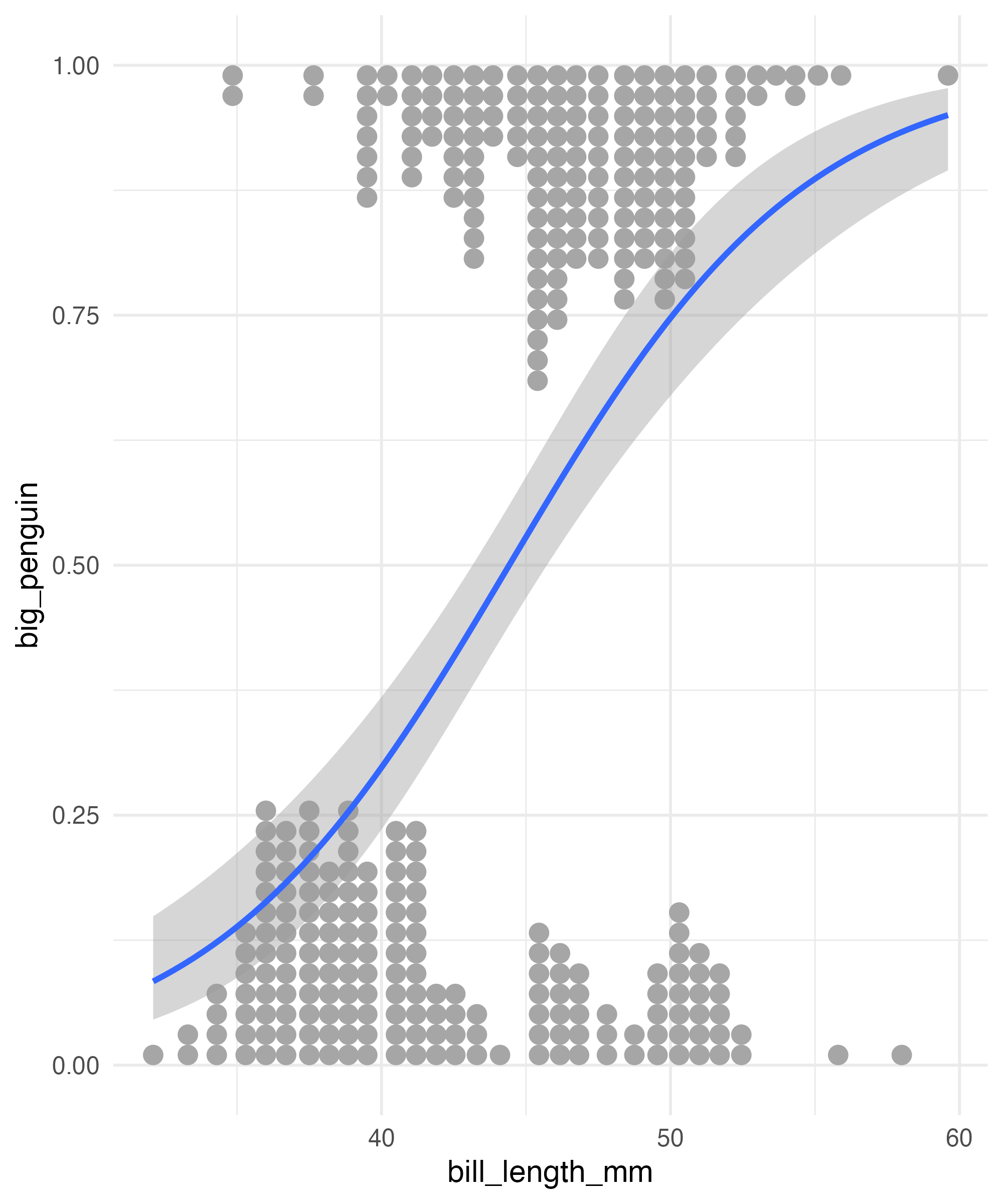
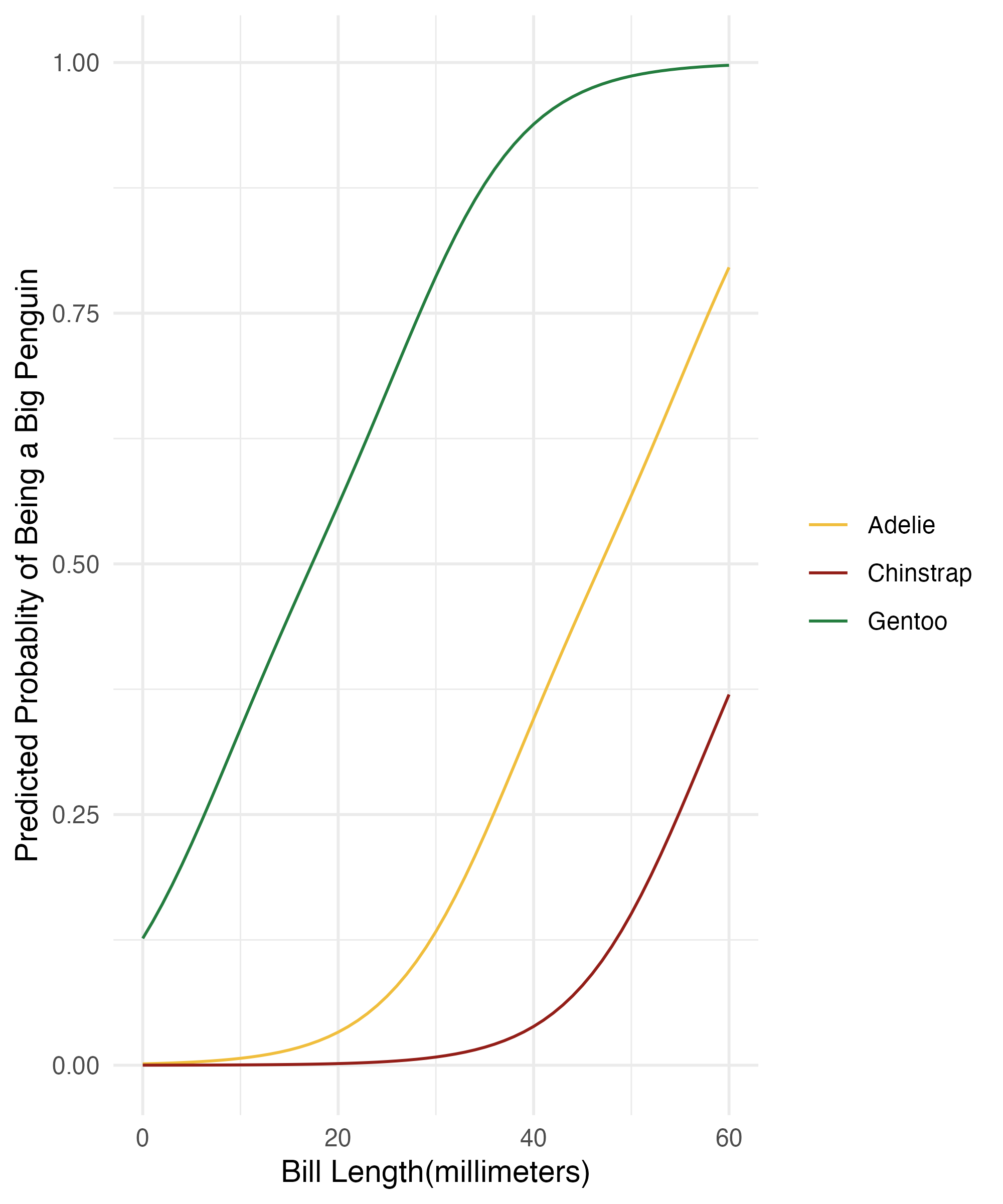
Since our coefficients in our logit model are uninterpretable we need to get some interpretable quantities. We can either use odds ratios by just doing exponeniate.

This is fine if your discipline does this. Political scientists especially prefer using average marginal effects.

Under the hood what is going on is that marginal effects is going to plug in the each row into the model and generate predictions and calculates the slope. Then will basically average across them. So the effect is basically just the average across the fitted results.

User Specified Values

emmeans

predictions_emmeans = base_model |> 
 emmeans(~ bill_length_mm + species, var = "bill_length_mm",
                   at = list(bill_length_mm = seq(0, 60,1)),
                   regrid = "response", delta = 0.001) |> 
  as_tibble() 

colors_plot = c("#f0be3d", "#931e18", "#247d3f")

ggplot(predictions_emmeans, aes(x = bill_length_mm, y = prob, color = species)) +
  geom_line() + 
  labs(x = "Bill Length(millimeters)", y = "Predicted Probablity of Being a Big Penguin",
       color = NULL) +
  theme(legend.position = "bottom") +
  theme_minimal() +
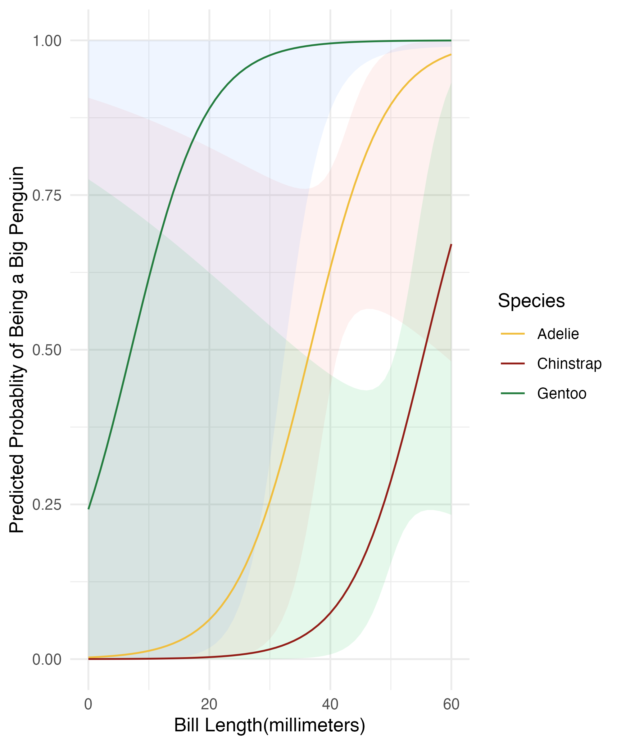
  scale_color_manual(values = colors_plot)

Marginal Effects

base_model_use = base_model |>
predictions(newdata = datagrid(bill_length_mm = c(0,61), 
                              species = unique))


plot_predictions(base_model,
                 condition = list("bill_length_mm" = 0:60,
                                   "species" = unique))  + 
  labs(x = "Bill Length(millimeters)", y = "Predicted Probablity of Being a Big Penguin",
       color = NULL) +
  theme(legend.position = "bottom") +
  theme_minimal() +
  scale_color_manual(values = colors_plot) +
  guides(fill = guide_legend(title = "Species", override.aes = list(fill = NA)),
         color = guide_legend(title = "Species",override.aes = list(fill = NA)))

Results

Machine Learning(basics)

Packages You Will Need

set.seed(1994) # make things reproducible
library(ISLR2)
library(caret)
library(leaps)
library(mlbench)
library(tidymodels) 
library(vip)

• Note caret and tidymodels have some namespace conflicts.
  • I personally would prefer to load one or the other

Tip

The Elements of Statistical Learning has all the R and Python code located at this website.

I generally am not a machine learning person. So I am just going to show you the basics of a machine learning workflow in R.

Creating Training and Test Sets

Caret

# Preprocess data  
peng =  penguins |> drop_na()

peng_caret = as.data.frame(peng)  

train_index_caret = caret::createDataPartition(peng_caret$body_mass_g, p = 0.7, list = FALSE, times = 1)

train_caret = peng_caret[train_index_caret,]

test_caret = peng_caret[-train_index_caret,]

Tidymodels

peng_models =  rsample::initial_split(peng, prop = 0.7)

peng_tidy_train = rsample::training(peng_models)

peng_tidy_test = rsample::testing(peng_models)

Create Cross Validations

Caret

peng_caret_cv = trainControl(method = "cv",
      number = 10)

Tidymodels

peng_cv_tidy = vfold_cv(peng_tidy_train, v = 10, strata = body_mass_g)

Fit a lasso regression

lasso_caret = train(body_mass_g ~ .,
                 data = train_caret,
                 method = "lasso",
                 trControl = peng_caret_cv)



tuning_grid_caret = data.frame(.fraction = 10^seq(-2, -1, length.out = 10))



lasso_caret_tune = train(body_mass_g ~ .,
                 data = train_caret,
                 method = "lasso",
                 trControl = peng_caret_cv,
                 tuneGrid = tuning_grid_caret)

predictions_caret = predict(lasso_caret_tune, newdata = test_caret)

All in all machine learning in R works. I just have not done it all that much. I have mostly done strucutural topic mo

Lasso Regression in Tidymodels

penguins_rec = recipe(body_mass_g ~ ., data = peng_tidy_test)  |>
step_center(all_predictors(), -all_nominal()) |>
step_dummy(all_nominal())

lasso_mod = linear_reg(mode = "regression",
                       penalty = tune(),
                       mixture = 1) |>
            set_engine("glmnet") # other package that fits lasso

wf = workflow() |>
add_model(lasso_mod) |>
add_recipe(penguins_rec)


my_grid = tibble(penalty = 10^seq(-2, -1, length.out = 10))


my_res = wf |>
tune_grid(resamples = peng_cv_tidy,
          grid = my_grid,
          control = control_grid(verbose = FALSE, save_pred = TRUE),
          metrics = metric_set(rmse))



good_mod = my_res |> select_best("rmse", maximize = FALSE)


final_fit = finalize_workflow(wf, good_mod) |>
fit(data = peng_tidy_train)


predict(final_fit, peng_tidy_test)

# A tibble: 100 × 1
   .pred
   <dbl>
 1 3377.
 2 3597.
 3 4102.
 4 3311.
 5 3343.
 6 4159.
 7 3655.
 8 3889.
 9 3540.
10 3895.
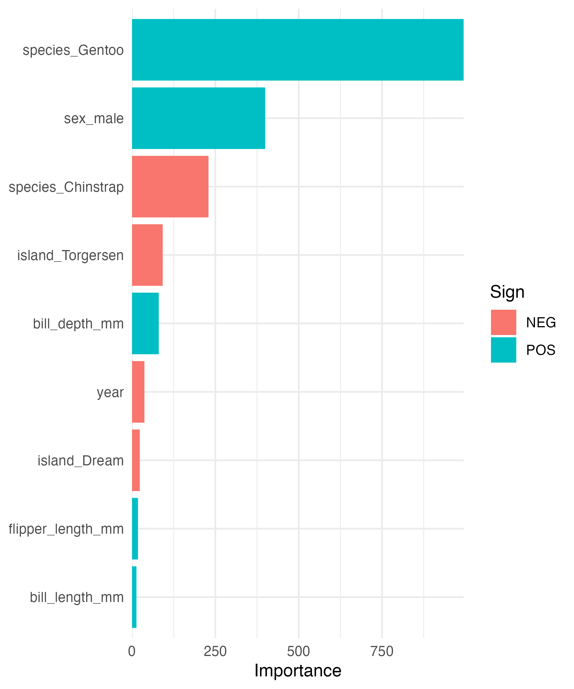
# … with 90 more rows

recipes, which is designed to help you preprocess your data before training your model. Recipes are built as a series of preprocessing steps, such as:

defines a model that can predict numeric values from predictors using a linear function. This function can fit regression models

is used to specify which package or system will be used to fit the model, along with any arguments specific to that software.

A workflow is a container object that aggregates information required to fit and predict from a model.

specifies the terms of the model and any preprocessing that is required through the usage of a recipe.

Variable Importance Plot

final_fit |>
fit(peng_tidy_train) |>
extract_fit_parsnip() |>
vi(lambda = good_mod$penalty) |>
mutate(
    Importance = abs(Importance),
    Variable = fct_reorder(Variable, Importance)
  ) |>
ggplot(aes(x = Importance,
          y = Variable,
         fill = Sign)) +
geom_col() +
scale_x_continuous(expand = c(0,0)) + 
labs(y = NULL) +
theme_minimal()