suppressPackageStartupMessages(library(tidyverse))
library(palmerpenguins)Translating What I know in the tidyverse to Python:
r
tidyverse
python
polars
This is me learning the snake language
Just a disclaimer. This is really just me working through the similarities and is going to be based on the tidyintelligence’s blog post, Robert Mitchell’s blog post, and Emily Rieder’s blog post. In all honesty, this is just for me to smash them together to have a one-stop shop for myself. If you found this post over these resources I highly recommend you check out these resources.
The Basics
As always we should load in the respective packages we are going to use.
import polars as pl
import polars.selectors as cs
from palmerpenguins import load_penguins

penguins = load_penguins().pipe(pl.from_pandas)


pl.Config(tbl_rows = 10)
<polars.config.Config object at 0x16858e660>Okay so far nothing too crazy! The main difference in loading in the packages and the data we are using is really just that to get with our familiar starts_with friends from the tidyverse we have to add polars.selectors and change some defaults. Lots of the time we would like to see the top and bottom portion and the column types. In R this is just our head, tail, glimpse/str in python it should be broadly similar.
head(penguins) |>
knitr::kable(booktabs = TRUE)| species | island | bill_length_mm | bill_depth_mm | flipper_length_mm | body_mass_g | sex | year |
|---|---|---|---|---|---|---|---|
| Adelie | Torgersen | 39.1 | 18.7 | 181 | 3750 | male | 2007 |
| Adelie | Torgersen | 39.5 | 17.4 | 186 | 3800 | female | 2007 |
| Adelie | Torgersen | 40.3 | 18.0 | 195 | 3250 | female | 2007 |
| Adelie | Torgersen | NA | NA | NA | NA | NA | 2007 |
| Adelie | Torgersen | 36.7 | 19.3 | 193 | 3450 | female | 2007 |
| Adelie | Torgersen | 39.3 | 20.6 | 190 | 3650 | male | 2007 |
penguins.head()
shape: (5, 8)
| species | island | bill_length_mm | bill_depth_mm | flipper_length_mm | body_mass_g | sex | year |
|---|---|---|---|---|---|---|---|
| str | str | f64 | f64 | f64 | f64 | str | i64 |
| "Adelie" | "Torgersen" | 39.1 | 18.7 | 181.0 | 3750.0 | "male" | 2007 |
| "Adelie" | "Torgersen" | 39.5 | 17.4 | 186.0 | 3800.0 | "female" | 2007 |
| "Adelie" | "Torgersen" | 40.3 | 18.0 | 195.0 | 3250.0 | "female" | 2007 |
| "Adelie" | "Torgersen" | null | null | null | null | null | 2007 |
| "Adelie" | "Torgersen" | 36.7 | 19.3 | 193.0 | 3450.0 | "female" | 2007 |
So one big difference for me is that when you are doing things with objects instead of feeding them directly to head you are doing object_name.head() which I suppose will take some time to get used to. I suppose for completeness we should look at the glimpse equivalent since I use that function all the time
glimpse(penguins)Rows: 344
Columns: 8
$ species <fct> Adelie, Adelie, Adelie, Adelie, Adelie, Adelie, Adel…
$ island <fct> Torgersen, Torgersen, Torgersen, Torgersen, Torgerse…
$ bill_length_mm <dbl> 39.1, 39.5, 40.3, NA, 36.7, 39.3, 38.9, 39.2, 34.1, …
$ bill_depth_mm <dbl> 18.7, 17.4, 18.0, NA, 19.3, 20.6, 17.8, 19.6, 18.1, …
$ flipper_length_mm <int> 181, 186, 195, NA, 193, 190, 181, 195, 193, 190, 186…
$ body_mass_g <int> 3750, 3800, 3250, NA, 3450, 3650, 3625, 4675, 3475, …
$ sex <fct> male, female, female, NA, female, male, female, male…
$ year <int> 2007, 2007, 2007, 2007, 2007, 2007, 2007, 2007, 2007…penguins.glimpse()Rows: 344
Columns: 8
$ species <str> 'Adelie', 'Adelie', 'Adelie', 'Adelie', 'Adelie', 'Adelie', 'Adelie', 'Adelie', 'Adelie', 'Adelie'
$ island <str> 'Torgersen', 'Torgersen', 'Torgersen', 'Torgersen', 'Torgersen', 'Torgersen', 'Torgersen', 'Torgersen', 'Torgersen', 'Torgersen'
$ bill_length_mm <f64> 39.1, 39.5, 40.3, null, 36.7, 39.3, 38.9, 39.2, 34.1, 42.0
$ bill_depth_mm <f64> 18.7, 17.4, 18.0, null, 19.3, 20.6, 17.8, 19.6, 18.1, 20.2
$ flipper_length_mm <f64> 181.0, 186.0, 195.0, null, 193.0, 190.0, 181.0, 195.0, 193.0, 190.0
$ body_mass_g <f64> 3750.0, 3800.0, 3250.0, null, 3450.0, 3650.0, 3625.0, 4675.0, 3475.0, 4250.0
$ sex <str> 'male', 'female', 'female', null, 'female', 'male', 'female', 'male', null, null
$ year <i64> 2007, 2007, 2007, 2007, 2007, 2007, 2007, 2007, 2007, 2007Okay! What is cool for me so far about polars is that it is more getting used to the whole . thing.
Filter
One of the key things in data cleaning or working with data is working with observations that fit some criteria! In this case, lets just grab all the rows that have Adelie penguins and are above the mean body mass
penguins |>
filter(species == "Adelie", body_mass_g > mean(body_mass_g, na.rm = TRUE))
# A tibble: 25 × 8
species island bill_length_mm bill_depth_mm flipper_length_mm body_mass_g
<fct> <fct> <dbl> <dbl> <int> <int>
1 Adelie Torgersen 39.2 19.6 195 4675
2 Adelie Torgersen 42 20.2 190 4250
3 Adelie Torgersen 34.6 21.1 198 4400
4 Adelie Torgersen 42.5 20.7 197 4500
5 Adelie Dream 39.8 19.1 184 4650
6 Adelie Dream 44.1 19.7 196 4400
7 Adelie Dream 39.6 18.8 190 4600
8 Adelie Biscoe 40.1 18.9 188 4300
9 Adelie Biscoe 41.3 21.1 195 4400
10 Adelie Torgersen 41.8 19.4 198 4450
# ℹ 15 more rows
# ℹ 2 more variables: sex <fct>, year <int>penguins.filter(pl.col("species") == "Adelie" &
pl.col("body_mass_g" > mean(pl.col("body_mass_g"))))NameError: name 'mean' is not definedThis is my first attempt at it! It looks like the problem I am running into is that Python does not have a base python where a function like mean is defined.
After fiddling with it for some time it turns out the filter call is actually not correctly defined either! So before each filter option, you need to add a set of ()
penguins |>
filter(species == "Adelie", body_mass_g > mean(body_mass_g, na.rm = TRUE))
# A tibble: 25 × 8
species island bill_length_mm bill_depth_mm flipper_length_mm body_mass_g
<fct> <fct> <dbl> <dbl> <int> <int>
1 Adelie Torgersen 39.2 19.6 195 4675
2 Adelie Torgersen 42 20.2 190 4250
3 Adelie Torgersen 34.6 21.1 198 4400
4 Adelie Torgersen 42.5 20.7 197 4500
5 Adelie Dream 39.8 19.1 184 4650
6 Adelie Dream 44.1 19.7 196 4400
7 Adelie Dream 39.6 18.8 190 4600
8 Adelie Biscoe 40.1 18.9 188 4300
9 Adelie Biscoe 41.3 21.1 195 4400
10 Adelie Torgersen 41.8 19.4 198 4450
# ℹ 15 more rows
# ℹ 2 more variables: sex <fct>, year <int>(penguins
.filter((pl.col("species") == "Adelie") &
(pl.col("body_mass_g") > pl.col("body_mass_g").mean())))
shape: (25, 8)
| species | island | bill_length_mm | bill_depth_mm | flipper_length_mm | body_mass_g | sex | year |
|---|---|---|---|---|---|---|---|
| str | str | f64 | f64 | f64 | f64 | str | i64 |
| "Adelie" | "Torgersen" | 39.2 | 19.6 | 195.0 | 4675.0 | "male" | 2007 |
| "Adelie" | "Torgersen" | 42.0 | 20.2 | 190.0 | 4250.0 | null | 2007 |
| "Adelie" | "Torgersen" | 34.6 | 21.1 | 198.0 | 4400.0 | "male" | 2007 |
| "Adelie" | "Torgersen" | 42.5 | 20.7 | 197.0 | 4500.0 | "male" | 2007 |
| "Adelie" | "Dream" | 39.8 | 19.1 | 184.0 | 4650.0 | "male" | 2007 |
| … | … | … | … | … | … | … | … |
| "Adelie" | "Biscoe" | 42.2 | 19.5 | 197.0 | 4275.0 | "male" | 2009 |
| "Adelie" | "Torgersen" | 41.5 | 18.3 | 195.0 | 4300.0 | "male" | 2009 |
| "Adelie" | "Dream" | 37.5 | 18.5 | 199.0 | 4475.0 | "male" | 2009 |
| "Adelie" | "Dream" | 39.7 | 17.9 | 193.0 | 4250.0 | "male" | 2009 |
| "Adelie" | "Dream" | 39.2 | 18.6 | 190.0 | 4250.0 | "male" | 2009 |
Nobody said this was going to be pretty or seamless! One other thing to get used to is that we are not going to be using something crazy like %in% for set membership! We use is_in
penguins |>
filter(species %in% c("Gentoo", "Chinstrap"),
       bill_depth_mm > median(bill_depth_mm, na.rm = TRUE))
# A tibble: 52 × 8
species island bill_length_mm bill_depth_mm flipper_length_mm body_mass_g
<fct> <fct> <dbl> <dbl> <int> <int>
1 Chinstrap Dream 46.5 17.9 192 3500
2 Chinstrap Dream 50 19.5 196 3900
3 Chinstrap Dream 51.3 19.2 193 3650
4 Chinstrap Dream 45.4 18.7 188 3525
5 Chinstrap Dream 52.7 19.8 197 3725
6 Chinstrap Dream 45.2 17.8 198 3950
7 Chinstrap Dream 46.1 18.2 178 3250
8 Chinstrap Dream 51.3 18.2 197 3750
9 Chinstrap Dream 46 18.9 195 4150
10 Chinstrap Dream 51.3 19.9 198 3700
# ℹ 42 more rows
# ℹ 2 more variables: sex <fct>, year <int>(
penguins
.filter((pl.col("species").is_in(["Chinstrap", "Gentoo"])) &
(pl.col("bill_depth_mm") > pl.col("bill_depth_mm").median()))
)
shape: (52, 8)
| species | island | bill_length_mm | bill_depth_mm | flipper_length_mm | body_mass_g | sex | year |
|---|---|---|---|---|---|---|---|
| str | str | f64 | f64 | f64 | f64 | str | i64 |
| "Chinstrap" | "Dream" | 46.5 | 17.9 | 192.0 | 3500.0 | "female" | 2007 |
| "Chinstrap" | "Dream" | 50.0 | 19.5 | 196.0 | 3900.0 | "male" | 2007 |
| "Chinstrap" | "Dream" | 51.3 | 19.2 | 193.0 | 3650.0 | "male" | 2007 |
| "Chinstrap" | "Dream" | 45.4 | 18.7 | 188.0 | 3525.0 | "female" | 2007 |
| "Chinstrap" | "Dream" | 52.7 | 19.8 | 197.0 | 3725.0 | "male" | 2007 |
| … | … | … | … | … | … | … | … |
| "Chinstrap" | "Dream" | 55.8 | 19.8 | 207.0 | 4000.0 | "male" | 2009 |
| "Chinstrap" | "Dream" | 43.5 | 18.1 | 202.0 | 3400.0 | "female" | 2009 |
| "Chinstrap" | "Dream" | 49.6 | 18.2 | 193.0 | 3775.0 | "male" | 2009 |
| "Chinstrap" | "Dream" | 50.8 | 19.0 | 210.0 | 4100.0 | "male" | 2009 |
| "Chinstrap" | "Dream" | 50.2 | 18.7 | 198.0 | 3775.0 | "female" | 2009 |
One other thing that is weird (to me at least) is that you do not have to set the polars functions to remove NA’s by default! Which I suppose is nice? But feels a bit wrong and weird to me as an R user.
A common case that you run into is that maybe there are a whole bunch of things or one thing that you don’t want. In R you would just add the neccessary negations ahead of what you want. In polars it is a little different if you want to exclude values from a set.
penguins |>
filter(!species %in% c("Gentoo", "Chinstrap"),
       island != "Dream")
# A tibble: 96 × 8
species island bill_length_mm bill_depth_mm flipper_length_mm body_mass_g
<fct> <fct> <dbl> <dbl> <int> <int>
1 Adelie Torgersen 39.1 18.7 181 3750
2 Adelie Torgersen 39.5 17.4 186 3800
3 Adelie Torgersen 40.3 18 195 3250
4 Adelie Torgersen NA NA NA NA
5 Adelie Torgersen 36.7 19.3 193 3450
6 Adelie Torgersen 39.3 20.6 190 3650
7 Adelie Torgersen 38.9 17.8 181 3625
8 Adelie Torgersen 39.2 19.6 195 4675
9 Adelie Torgersen 34.1 18.1 193 3475
10 Adelie Torgersen 42 20.2 190 4250
# ℹ 86 more rows
# ℹ 2 more variables: sex <fct>, year <int># | error: true
# | label: set-filter-not
penguins.filter((pl.col("species").is_in(["Chinstrap", "Gentoo"]).not_()) &
(pl.col("island") != 'Dream'))
shape: (96, 8)
| species | island | bill_length_mm | bill_depth_mm | flipper_length_mm | body_mass_g | sex | year |
|---|---|---|---|---|---|---|---|
| str | str | f64 | f64 | f64 | f64 | str | i64 |
| "Adelie" | "Torgersen" | 39.1 | 18.7 | 181.0 | 3750.0 | "male" | 2007 |
| "Adelie" | "Torgersen" | 39.5 | 17.4 | 186.0 | 3800.0 | "female" | 2007 |
| "Adelie" | "Torgersen" | 40.3 | 18.0 | 195.0 | 3250.0 | "female" | 2007 |
| "Adelie" | "Torgersen" | null | null | null | null | null | 2007 |
| "Adelie" | "Torgersen" | 36.7 | 19.3 | 193.0 | 3450.0 | "female" | 2007 |
| … | … | … | … | … | … | … | … |
| "Adelie" | "Torgersen" | 41.5 | 18.3 | 195.0 | 4300.0 | "male" | 2009 |
| "Adelie" | "Torgersen" | 39.0 | 17.1 | 191.0 | 3050.0 | "female" | 2009 |
| "Adelie" | "Torgersen" | 44.1 | 18.0 | 210.0 | 4000.0 | "male" | 2009 |
| "Adelie" | "Torgersen" | 38.5 | 17.9 | 190.0 | 3325.0 | "female" | 2009 |
| "Adelie" | "Torgersen" | 43.1 | 19.2 | 197.0 | 3500.0 | "male" | 2009 |
Select
In some cases, we have a dataset with extraneous columns we do not care for. Let’s do a really extreme example
penguins |>
select(island)
# A tibble: 344 × 1
island
<fct>
1 Torgersen
2 Torgersen
3 Torgersen
4 Torgersen
5 Torgersen
6 Torgersen
7 Torgersen
8 Torgersen
9 Torgersen
10 Torgersen
# ℹ 334 more rowspenguins.select((pl.col("island")))
shape: (344, 1)
| island |
|---|
| str |
| "Torgersen" |
| "Torgersen" |
| "Torgersen" |
| "Torgersen" |
| "Torgersen" |
| … |
| "Dream" |
| "Dream" |
| "Dream" |
| "Dream" |
| "Dream" |
OKAY! first try now we are cooking! If we wanted to do multiple columns we would do something to the effect of
penguins |>
select(species, island)
# A tibble: 344 × 2
species island
<fct> <fct>
1 Adelie Torgersen
2 Adelie Torgersen
3 Adelie Torgersen
4 Adelie Torgersen
5 Adelie Torgersen
6 Adelie Torgersen
7 Adelie Torgersen
8 Adelie Torgersen
9 Adelie Torgersen
10 Adelie Torgersen
# ℹ 334 more rowsTo do multiple columns we could do something to the effect of this:
penguins.select((pl.col("species", "island")))
shape: (344, 2)
| species | island |
|---|---|
| str | str |
| "Adelie" | "Torgersen" |
| "Adelie" | "Torgersen" |
| "Adelie" | "Torgersen" |
| "Adelie" | "Torgersen" |
| "Adelie" | "Torgersen" |
| … | … |
| "Chinstrap" | "Dream" |
| "Chinstrap" | "Dream" |
| "Chinstrap" | "Dream" |
| "Chinstrap" | "Dream" |
| "Chinstrap" | "Dream" |
Which feels more natural to me, but to some extent a dictionary would probably be more pythony. One thing I use all the time is using tidyselectors like starts_with
Using Selectors
penguins |>
select(starts_with("bill"))
# A tibble: 344 × 2
bill_length_mm bill_depth_mm
<dbl> <dbl>
1 39.1 18.7
2 39.5 17.4
3 40.3 18
4 NA NA
5 36.7 19.3
6 39.3 20.6
7 38.9 17.8
8 39.2 19.6
9 34.1 18.1
10 42 20.2
# ℹ 334 more rowspenguins.select(cs.starts_with("bill"))
shape: (344, 2)
| bill_length_mm | bill_depth_mm |
|---|---|
| f64 | f64 |
| 39.1 | 18.7 |
| 39.5 | 17.4 |
| 40.3 | 18.0 |
| null | null |
| 36.7 | 19.3 |
| … | … |
| 55.8 | 19.8 |
| 43.5 | 18.1 |
| 49.6 | 18.2 |
| 50.8 | 19.0 |
| 50.2 | 18.7 |
This is actually so cool that in this case it works exactly like the tidyverse selector functions!
Renaming Columns
I am a simple man I like snake_case but lets say I am more camel case inclined. I may want to rename columns that I am using as to not deal with object not found messages because I am used to typing billLengthMm. In the tidyverse we would do
penguins |>
rename(BillLengthMm = bill_length_mm,
       BillDepthMm = bill_depth_mm)
# A tibble: 344 × 8
species island BillLengthMm BillDepthMm flipper_length_mm body_mass_g sex
<fct> <fct> <dbl> <dbl> <int> <int> <fct>
1 Adelie Torgers… 39.1 18.7 181 3750 male
2 Adelie Torgers… 39.5 17.4 186 3800 fema…
3 Adelie Torgers… 40.3 18 195 3250 fema…
4 Adelie Torgers… NA NA NA NA <NA>
5 Adelie Torgers… 36.7 19.3 193 3450 fema…
6 Adelie Torgers… 39.3 20.6 190 3650 male
7 Adelie Torgers… 38.9 17.8 181 3625 fema…
8 Adelie Torgers… 39.2 19.6 195 4675 male
9 Adelie Torgers… 34.1 18.1 193 3475 <NA>
10 Adelie Torgers… 42 20.2 190 4250 <NA>
# ℹ 334 more rows
# ℹ 1 more variable: year <int>penguins = penguins.rename({"bill_length_mm":"BillLengthMm",
"bill_depth_mm":"BillDepthMm"})
penguins = penguins.rename({"BillLengthMm": "bill_length_mm",
"BillDepthMm":"bill_depth_mm"})In effect the thing you need to switch in your head when working in polars is that the order goes old_name:new_name I assigned it to an object because I wanted to test out a module I found online.
Mutate
Okay we have worked with subsets now we need to actually create some things. We should also work on chaining things together. Lets first with doing math stuff to the columns. Lets start with how I think it works in polars and if it errors then we can go and fix it
penguins |>
mutate(sqr_bill_length = bill_length_mm^2) |>
select(sqr_bill_length) |>
head()
# A tibble: 6 × 1
sqr_bill_length
<dbl>
1 1529.
2 1560.
3 1624.
4 NA
5 1347.
6 1544.penguins.mutate({pl.col("bill_length_mm")^2: "sqr_bill_length"}).select(pl.col("sqr_bill_length"))AttributeError: 'DataFrame' object has no attribute 'mutate'Okay where I am coming from is that in my head what we are doing is using the same logic as renaming columns. Lets fix it. So the first problem is that there is no mutate verb. Instead we use with_column
penguins.with_columns(sqr_bill_length = pl.col("bill_length_mm")**2).select(pl.col("sqr_bill_length")).head()
shape: (5, 1)
| sqr_bill_length |
|---|
| f64 |
| 1528.81 |
| 1560.25 |
| 1624.09 |
| null |
| 1346.89 |
Okay this is the general idea. One of the big advantages of mutate is that we chain things together in the same mutate col. So lets say we wanted to square something than return it back to the original value
penguins |>
mutate(sqr_bill = bill_length_mm^2,
       og_bill = sqrt(sqr_bill)) |>
       select(sqr_bill, og_bill, bill_length_mm) |>
       head(n = 5)
# A tibble: 5 × 3
sqr_bill og_bill bill_length_mm
<dbl> <dbl> <dbl>
1 1529. 39.1 39.1
2 1560. 39.5 39.5
3 1624. 40.3 40.3
4 NA NA NA
5 1347. 36.7 36.7penguins.with_columns(sqr_bill = pl.col("bill_length_mm")**2).with_columns(og_bill = pl.col("sqr_bill").sqrt()).select(pl.col("sqr_bill", "og_bill", "bill_length_mm")).head(5)
shape: (5, 3)
| sqr_bill | og_bill | bill_length_mm |
|---|---|---|
| f64 | f64 | f64 |
| 1528.81 | 39.1 | 39.1 |
| 1560.25 | 39.5 | 39.5 |
| 1624.09 | 40.3 | 40.3 |
| null | null | null |
| 1346.89 | 36.7 | 36.7 |
Now the next step is creating conditionals
ifelse equivalents
penguins |>
mutate(female = ifelse(sex == "female", TRUE, FALSE)) |>
select(sex, female) |>
head(5)
# A tibble: 5 × 2
sex female
<fct> <lgl>
1 male FALSE
2 female TRUE
3 female TRUE
4 <NA> NA
5 female TRUE # | label: check
penguins.with_columns(female=pl.when(pl.col("sex") == "female").then(
True).otherwise(False)).select(["sex", "female"]).head(5)
shape: (5, 2)
| sex | female |
|---|---|
| str | bool |
| "male" | false |
| "female" | true |
| "female" | true |
| null | false |
| "female" | true |
Full disclosure this took a much longer time than shown but this is the basic idea. Lets do this to keep myself a bit more honest. Recreate a silly example that I use to teach ifelse using the starwars dataset.
data("starwars")

arrow::write_parquet(starwars, "starwars.parquet")starwars |>
mutate(dog_years = birth_year * 7,
comment = paste(name, "is", dog_years, "in dog years")) |>
select(name, dog_years, comment) |>
head(5)# A tibble: 5 × 3
name dog_years comment
<chr> <dbl> <chr>
1 Luke Skywalker 133 Luke Skywalker is 133 in dog years
2 C-3PO 784 C-3PO is 784 in dog years
3 R2-D2 231 R2-D2 is 231 in dog years
4 Darth Vader 293. Darth Vader is 293.3 in dog years
5 Leia Organa 133 Leia Organa is 133 in dog years starwars = pl.read_parquet("starwars.parquet")
starwars.with_columns(dog_years=pl.col("birth_year") * 7).with_columns(dog_years_string=pl.col("dog_years").cast(
str)).with_columns(pl.concat_str([pl.col('name') , pl.lit('is'), pl.col('dog_years_string') , pl.lit('in dog years')]).alias('character_age')).select(pl.col('character_age'))
shape: (87, 1)
| character_age |
|---|
| str |
| "Luke Skywalkeris133.0in dog ye… |
| "C-3POis784.0in dog years" |
| "R2-D2is231.0in dog years" |
| "Darth Vaderis293.3in dog years" |
| "Leia Organais133.0in dog years" |
| … |
| null |
| null |
| null |
| null |
| null |
penguins.with_columns(big_peng = pl.when(pl.col("body_mass_g") > pl.col("body_mass_g").mean()).then(True).otherwise(False))
shape: (344, 9)
| species | island | bill_length_mm | bill_depth_mm | flipper_length_mm | body_mass_g | sex | year | big_peng |
|---|---|---|---|---|---|---|---|---|
| str | str | f64 | f64 | f64 | f64 | str | i64 | bool |
| "Adelie" | "Torgersen" | 39.1 | 18.7 | 181.0 | 3750.0 | "male" | 2007 | false |
| "Adelie" | "Torgersen" | 39.5 | 17.4 | 186.0 | 3800.0 | "female" | 2007 | false |
| "Adelie" | "Torgersen" | 40.3 | 18.0 | 195.0 | 3250.0 | "female" | 2007 | false |
| "Adelie" | "Torgersen" | null | null | null | null | null | 2007 | false |
| "Adelie" | "Torgersen" | 36.7 | 19.3 | 193.0 | 3450.0 | "female" | 2007 | false |
| … | … | … | … | … | … | … | … | … |
| "Chinstrap" | "Dream" | 55.8 | 19.8 | 207.0 | 4000.0 | "male" | 2009 | false |
| "Chinstrap" | "Dream" | 43.5 | 18.1 | 202.0 | 3400.0 | "female" | 2009 | false |
| "Chinstrap" | "Dream" | 49.6 | 18.2 | 193.0 | 3775.0 | "male" | 2009 | false |
| "Chinstrap" | "Dream" | 50.8 | 19.0 | 210.0 | 4100.0 | "male" | 2009 | false |
| "Chinstrap" | "Dream" | 50.2 | 18.7 | 198.0 | 3775.0 | "female" | 2009 | false |
Multiple columns
So one of the rubbing points as a dplyr user was that with columns isn’t always easy to use if you want to refer to columns you made previously. However, I found that you can use the trusty old walrus operator := to do that.
penguins.with_columns(
    body_mass_g := pl.col('body_mass_g')**2,
    pl.col('body_mass_g').sqrt().alias('bg')
)
shape: (344, 9)
| species | island | bill_length_mm | bill_depth_mm | flipper_length_mm | body_mass_g | sex | year | bg |
|---|---|---|---|---|---|---|---|---|
| str | str | f64 | f64 | f64 | f64 | str | i64 | f64 |
| "Adelie" | "Torgersen" | 39.1 | 18.7 | 181.0 | 1.40625e7 | "male" | 2007 | 61.237244 |
| "Adelie" | "Torgersen" | 39.5 | 17.4 | 186.0 | 1.444e7 | "female" | 2007 | 61.64414 |
| "Adelie" | "Torgersen" | 40.3 | 18.0 | 195.0 | 1.05625e7 | "female" | 2007 | 57.008771 |
| "Adelie" | "Torgersen" | null | null | null | null | null | 2007 | null |
| "Adelie" | "Torgersen" | 36.7 | 19.3 | 193.0 | 1.19025e7 | "female" | 2007 | 58.736701 |
| … | … | … | … | … | … | … | … | … |
| "Chinstrap" | "Dream" | 55.8 | 19.8 | 207.0 | 1.6e7 | "male" | 2009 | 63.245553 |
| "Chinstrap" | "Dream" | 43.5 | 18.1 | 202.0 | 1.156e7 | "female" | 2009 | 58.309519 |
| "Chinstrap" | "Dream" | 49.6 | 18.2 | 193.0 | 1.4250625e7 | "male" | 2009 | 61.441029 |
| "Chinstrap" | "Dream" | 50.8 | 19.0 | 210.0 | 1.681e7 | "male" | 2009 | 64.031242 |
| "Chinstrap" | "Dream" | 50.2 | 18.7 | 198.0 | 1.4250625e7 | "female" | 2009 | 61.441029 |
In this case we are just modifying things in place and then simply transforming things back.
Group by and summarize
Last but not least we need to do the group by and summarise bit. It looks like this is slightly more intuitive
penguins |>
group_by(species) |>
summarise(total = n())
# A tibble: 3 × 2
species total
<fct> <int>
1 Adelie 152
2 Chinstrap 68
3 Gentoo 124penguins.group_by(pl.col("species")).agg(total = pl.count())
shape: (3, 2)
| species | total |
|---|---|
| str | u32 |
| "Chinstrap" | 68 |
| "Gentoo" | 124 |
| "Adelie" | 152 |
Lets do some mathy stuff
penguins.group_by(pl.col("species")).agg(count = pl.len(),
                                         mean_flipp = pl.mean("flipper_length_mm"),
                                         median_flipp = pl.median("flipper_length_mm"))
shape: (3, 4)
| species | count | mean_flipp | median_flipp |
|---|---|---|---|
| str | u32 | f64 | f64 |
| "Gentoo" | 124 | 217.186992 | 216.0 |
| "Chinstrap" | 68 | 195.823529 | 196.0 |
| "Adelie" | 152 | 189.953642 | 190.0 |
across
A thing that is useful in summarize is that we can use our selectors to summarise across multiple columns like this
penguins |>
group_by(species) |>
summarise(across(starts_with("bill"), list(mean = \(x) mean(x, na.rm = TRUE,
                                           median = \(x) median(x, na.rm,  TRUE)))))
# A tibble: 3 × 3
species bill_length_mm_mean bill_depth_mm_mean
<fct> <dbl> <dbl>
1 Adelie 38.8 18.3
2 Chinstrap 48.8 18.4
3 Gentoo 47.5 15.0In polars I imagine it would probably be something like this
penguins.group_by(pl.col("species")).agg(cs.starts_with("bill").mean())
shape: (3, 3)
| species | bill_length_mm | bill_depth_mm |
|---|---|---|
| str | f64 | f64 |
| "Adelie" | 38.791391 | 18.346358 |
| "Gentoo" | 47.504878 | 14.982114 |
| "Chinstrap" | 48.833824 | 18.420588 |
The think I am running into now is that I would like to add a _ without doing any extra work. It looks like according to the docs it should be this
penguins.group_by(pl.col("species")).agg(cs.starts_with("bill").mean().name.suffix("_mean"),
                                         cs.starts_with("bill").median().name.suffix("_median"))
shape: (3, 5)
| species | bill_length_mm_mean | bill_depth_mm_mean | bill_length_mm_median | bill_depth_mm_median |
|---|---|---|---|---|
| str | f64 | f64 | f64 | f64 |
| "Gentoo" | 47.504878 | 14.982114 | 47.3 | 15.0 |
| "Adelie" | 38.791391 | 18.346358 | 38.8 | 18.4 |
| "Chinstrap" | 48.833824 | 18.420588 | 49.55 | 18.45 |
Joins in Polars
It would be nice if we had all the data we wanted in one dataset but that is not life we often need to join data. Critically we also would not want to have all our data in one place if we care about users safety. So we may want to keep portions of the dataset in separate places. So lets define a simple dataset to work with.
national_data <- tribble(
  ~state, ~year, ~unemployment, ~inflation, ~population,
  "GA",   2018,  5,             2,          100,
  "GA",   2019,  5.3,           1.8,        200,
  "GA",   2020,  5.2,           2.5,        300,
  "NC",   2018,  6.1,           1.8,        350,
  "NC",   2019,  5.9,           1.6,        375,
  "NC",   2020,  5.3,           1.8,        400,
  "CO",   2018,  4.7,           2.7,        200,
  "CO",   2019,  4.4,           2.6,        300,
  "CO",   2020,  5.1,           2.5,        400
)

national_libraries <- tribble(
  ~state, ~year, ~libraries, ~schools,
  "CO",   2018,  230,        470,
  "CO",   2019,  240,        440,
  "CO",   2020,  270,        510,
  "NC",   2018,  200,        610,
  "NC",   2019,  210,        590,
  "NC",   2020,  220,        530,
)
national_dict = {"state": ["Ga", "Ga", "Ga",  "NC", "NC", "NC", "CO", "CO", "CO"], "unemployment":[6,6,8,6,4,3,7,8,9], "year": [2019,2018,2017,2019,2018,2017,2019,2018,2017]}


national_data = pl.DataFrame(national_dict)


library_dict = {"state":["CO", "CO", "CO"], "libraries": [23234,2343234,32342342], "year":[2019,2018,2017]}


library_data = pl.DataFrame(library_dict)
We may want to merge in the library dataset. In tidyland we would do something like this
national_data |>
left_join(national_libraries, join_by(state, year))
# A tibble: 9 × 7
state year unemployment inflation population libraries schools
<chr> <dbl> <dbl> <dbl> <dbl> <dbl> <dbl>
1 GA 2018 5 2 100 NA NA
2 GA 2019 5.3 1.8 200 NA NA
3 GA 2020 5.2 2.5 300 NA NA
4 NC 2018 6.1 1.8 350 200 610
5 NC 2019 5.9 1.6 375 210 590
6 NC 2020 5.3 1.8 400 220 530
7 CO 2018 4.7 2.7 200 230 470
8 CO 2019 4.4 2.6 300 240 440
9 CO 2020 5.1 2.5 400 270 510In polars land we would join the data like this
joined_data = national_data.join(library_data, on = ["state","year"], how = "left")

joined_data
shape: (9, 4)
| state | unemployment | year | libraries |
|---|---|---|---|
| str | i64 | i64 | i64 |
| "Ga" | 6 | 2019 | null |
| "Ga" | 6 | 2018 | null |
| "Ga" | 8 | 2017 | null |
| "NC" | 6 | 2019 | null |
| "NC" | 4 | 2018 | null |
| "NC" | 3 | 2017 | null |
| "CO" | 7 | 2019 | 23234 |
| "CO" | 8 | 2018 | 2343234 |
| "CO" | 9 | 2017 | 32342342 |
This is honestly pretty comfortable. One thing that is really nice about dplyr is that you can pretty easily join columns that are not named the same thing.
national_libraries = national_libraries |>
rename(state_name = state)


national_data |>
left_join(national_libraries, join_by(state == state_name, year))
# A tibble: 9 × 7
state year unemployment inflation population libraries schools
<chr> <dbl> <dbl> <dbl> <dbl> <dbl> <dbl>
1 GA 2018 5 2 100 NA NA
2 GA 2019 5.3 1.8 200 NA NA
3 GA 2020 5.2 2.5 300 NA NA
4 NC 2018 6.1 1.8 350 200 610
5 NC 2019 5.9 1.6 375 210 590
6 NC 2020 5.3 1.8 400 220 530
7 CO 2018 4.7 2.7 200 230 470
8 CO 2019 4.4 2.6 300 240 440
9 CO 2020 5.1 2.5 400 270 510In polars the process is less clear immediately. Instead of a nice join_by argument you have specify the keys separately. But still pretty intuitive.
library_dat = library_data.rename({"state": "state_name"})


national_data.join(library_dat, left_on = ["state", "year"],
               right_on = ["state_name", "year"], how = "left" )
shape: (9, 4)
| state | unemployment | year | libraries |
|---|---|---|---|
| str | i64 | i64 | i64 |
| "Ga" | 6 | 2019 | null |
| "Ga" | 6 | 2018 | null |
| "Ga" | 8 | 2017 | null |
| "NC" | 6 | 2019 | null |
| "NC" | 4 | 2018 | null |
| "NC" | 3 | 2017 | null |
| "CO" | 7 | 2019 | 23234 |
| "CO" | 8 | 2018 | 2343234 |
| "CO" | 9 | 2017 | 32342342 |
Binding Rows
Sometimes we just want to add rows to our data
a = data.frame(id = 1:2, vals = 1:2)

b  = data.frame(id = 3:4, vals = 3:4)


a |>
bind_rows(b)
id vals
1 1 1
2 2 2
3 3 3
4 4 4or we want to add columns
c = data.frame(chars = c("hello", "lorem"),
               var_23 = c("world", "ipsum"))

a |>
bind_cols(c)
id vals chars var_23
1 1 1 hello world
2 2 2 lorem ipsumHow would we do this in polars?
a = pl.DataFrame(
       {"a": [1,2],
        "b": [3,4]}
)

b = pl.DataFrame({"a" : [3,4], "b": [5,6]})


pl.concat([a, b], how = "vertical")
shape: (4, 2)
| a | b |
|---|---|
| i64 | i64 |
| 1 | 3 |
| 2 | 4 |
| 3 | 5 |
| 4 | 6 |
Again fairly intuitive if we wanted to bind the columns
c = pl.DataFrame({"chars": ["hello", "lorem"], "chars2":["world","ipsum"]})


pl.concat([a,c], how = "horizontal")
shape: (2, 4)
| a | b | chars | chars2 |
|---|---|---|---|
| i64 | i64 | str | str |
| 1 | 3 | "hello" | "world" |
| 2 | 4 | "lorem" | "ipsum" |
Tidyr
Pivots of all shapes
Sometimes we need to pivot our data. Lets use the built in example from tidyr. Basically we have a whole bunch of columns that denote counts of income brackets
relig = relig_income


write_csv(relig,"relig_income.csv")


head(relig_income)
# A tibble: 6 × 11
religion `<$10k` `$10-20k` `$20-30k` `$30-40k` `$40-50k` `$50-75k` `$75-100k`
<chr> <dbl> <dbl> <dbl> <dbl> <dbl> <dbl> <dbl>
1 Agnostic 27 34 60 81 76 137 122
2 Atheist 12 27 37 52 35 70 73
3 Buddhist 27 21 30 34 33 58 62
4 Catholic 418 617 732 670 638 1116 949
5 Don’t kn… 15 14 15 11 10 35 21
6 Evangeli… 575 869 1064 982 881 1486 949
# ℹ 3 more variables: `$100-150k` <dbl>, `>150k` <dbl>,
# `Don't know/refused` <dbl>In tidyr we would just do this
relig |>
pivot_longer(-religion,
              names_to = "income_bracket",
              values_to = "count")
# A tibble: 180 × 3
religion income_bracket count
<chr> <chr> <dbl>
1 Agnostic <$10k 27
2 Agnostic $10-20k 34
3 Agnostic $20-30k 60
4 Agnostic $30-40k 81
5 Agnostic $40-50k 76
6 Agnostic $50-75k 137
7 Agnostic $75-100k 122
8 Agnostic $100-150k 109
9 Agnostic >150k 84
10 Agnostic Don't know/refused 96
# ℹ 170 more rowswhich is nice because we can just identify a column and then pivot. One thing that I will have to just memorize is that when we are moving things to long in polars than we melt the dataframe. Kind of like a popsicle or something. The mnemonic device will come to me eventually
relig = pl.read_csv("relig_income.csv")

relig.head()
shape: (5, 11)
| religion | <$10k | $10-20k | $20-30k | $30-40k | $40-50k | $50-75k | $75-100k | $100-150k | >150k | Don't know/refused |
|---|---|---|---|---|---|---|---|---|---|---|
| str | i64 | i64 | i64 | i64 | i64 | i64 | i64 | i64 | i64 | i64 |
| "Agnostic" | 27 | 34 | 60 | 81 | 76 | 137 | 122 | 109 | 84 | 96 |
| "Atheist" | 12 | 27 | 37 | 52 | 35 | 70 | 73 | 59 | 74 | 76 |
| "Buddhist" | 27 | 21 | 30 | 34 | 33 | 58 | 62 | 39 | 53 | 54 |
| "Catholic" | 418 | 617 | 732 | 670 | 638 | 1116 | 949 | 792 | 633 | 1489 |
| "Don’t know/refused" | 15 | 14 | 15 | 11 | 10 | 35 | 21 | 17 | 18 | 116 |
To melt all we do is
relig.melt(id_vars = "religion", variable_name = "income_bracket", value_name = "count")
shape: (180, 3)
| religion | income_bracket | count |
|---|---|---|
| str | str | i64 |
| "Agnostic" | "<$10k" | 27 |
| "Atheist" | "<$10k" | 12 |
| "Buddhist" | "<$10k" | 27 |
| "Catholic" | "<$10k" | 418 |
| "Don’t know/refused" | "<$10k" | 15 |
| … | … | … |
| "Orthodox" | "Don't know/refused" | 73 |
| "Other Christian" | "Don't know/refused" | 18 |
| "Other Faiths" | "Don't know/refused" | 71 |
| "Other World Religions" | "Don't know/refused" | 8 |
| "Unaffiliated" | "Don't know/refused" | 597 |
same would go for the pivoting wider
penguins.pivot(index = "island",columns = "species", values = "body_mass_g",
              aggregate_function="sum")
shape: (3, 4)
| island | Adelie | Gentoo | Chinstrap |
|---|---|---|---|
| str | f64 | f64 | f64 |
| "Torgersen" | 189025.0 | 0.0 | 0.0 |
| "Biscoe" | 163225.0 | 624350.0 | 0.0 |
| "Dream" | 206550.0 | 0.0 | 253850.0 |
this isn’t quite the same because we are aggregating it. This is likely just a skill issue on the user end. But still we have wide data now!
Using selectors in pivot longer
A slightly more complex example is using the billboards datas
billboards = tidyr::billboard


write_csv(billboards, "billboard.csv")


head(billboards)
# A tibble: 6 × 79
artist track date.entered wk1 wk2 wk3 wk4 wk5 wk6 wk7 wk8
<chr> <chr> <date> <dbl> <dbl> <dbl> <dbl> <dbl> <dbl> <dbl> <dbl>
1 2 Pac Baby… 2000-02-26 87 82 72 77 87 94 99 NA
2 2Ge+her The … 2000-09-02 91 87 92 NA NA NA NA NA
3 3 Doors Do… Kryp… 2000-04-08 81 70 68 67 66 57 54 53
4 3 Doors Do… Loser 2000-10-21 76 76 72 69 67 65 55 59
5 504 Boyz Wobb… 2000-04-15 57 34 25 17 17 31 36 49
6 98^0 Give… 2000-08-19 51 39 34 26 26 19 2 2
# ℹ 68 more variables: wk9 <dbl>, wk10 <dbl>, wk11 <dbl>, wk12 <dbl>,
# wk13 <dbl>, wk14 <dbl>, wk15 <dbl>, wk16 <dbl>, wk17 <dbl>, wk18 <dbl>,
# wk19 <dbl>, wk20 <dbl>, wk21 <dbl>, wk22 <dbl>, wk23 <dbl>, wk24 <dbl>,
# wk25 <dbl>, wk26 <dbl>, wk27 <dbl>, wk28 <dbl>, wk29 <dbl>, wk30 <dbl>,
# wk31 <dbl>, wk32 <dbl>, wk33 <dbl>, wk34 <dbl>, wk35 <dbl>, wk36 <dbl>,
# wk37 <dbl>, wk38 <dbl>, wk39 <dbl>, wk40 <dbl>, wk41 <dbl>, wk42 <dbl>,
# wk43 <dbl>, wk44 <dbl>, wk45 <dbl>, wk46 <dbl>, wk47 <dbl>, wk48 <dbl>, … billboards |>
pivot_longer(cols = starts_with("wk"),
names_to = "week",
values_to = "count_of_weeks")# A tibble: 24,092 × 5
artist track date.entered week count_of_weeks
<chr> <chr> <date> <chr> <dbl>
1 2 Pac Baby Don't Cry (Keep... 2000-02-26 wk1 87
2 2 Pac Baby Don't Cry (Keep... 2000-02-26 wk2 82
3 2 Pac Baby Don't Cry (Keep... 2000-02-26 wk3 72
4 2 Pac Baby Don't Cry (Keep... 2000-02-26 wk4 77
5 2 Pac Baby Don't Cry (Keep... 2000-02-26 wk5 87
6 2 Pac Baby Don't Cry (Keep... 2000-02-26 wk6 94
7 2 Pac Baby Don't Cry (Keep... 2000-02-26 wk7 99
8 2 Pac Baby Don't Cry (Keep... 2000-02-26 wk8 NA
9 2 Pac Baby Don't Cry (Keep... 2000-02-26 wk9 NA
10 2 Pac Baby Don't Cry (Keep... 2000-02-26 wk10 NA
# ℹ 24,082 more rowsWe can do something similar with polars by using our selectors.
billboards = pl.read_csv("billboard.csv")


billboards.melt(id_vars = "artist",value_vars  = cs.starts_with("wk"),
                variable_name = "week", value_name = "count" )
shape: (24_092, 3)
| artist | week | count |
|---|---|---|
| str | str | str |
| "2 Pac" | "wk1" | "87" |
| "2Ge+her" | "wk1" | "91" |
| "3 Doors Down" | "wk1" | "81" |
| "3 Doors Down" | "wk1" | "76" |
| "504 Boyz" | "wk1" | "57" |
| … | … | … |
| "Yankee Grey" | "wk76" | "NA" |
| "Yearwood, Trisha" | "wk76" | "NA" |
| "Ying Yang Twins" | "wk76" | "NA" |
| "Zombie Nation" | "wk76" | "NA" |
| "matchbox twenty" | "wk76" | "NA" |
Broadly it works the same but if you don’t specify the id vars you will end up with just the week and count column
Unnest
Sometimes we have these unfriendly list columns that we would like to make not lists. Lets go ahead and use the starwars list columns.
starwars_lists = starwars |>
select(name, where(is.list)) |>
unnest_longer(starships , keep_empty = TRUE) |>
unnest_longer(films, keep_empty = TRUE) |>
unnest_longer(vehicles, keep_empty = TRUE)


head(starwars_lists)
# A tibble: 6 × 4
name films vehicles starships
<chr> <chr> <chr> <chr>
1 Luke Skywalker A New Hope Snowspeeder X-wing
2 Luke Skywalker A New Hope Imperial Speeder Bike X-wing
3 Luke Skywalker The Empire Strikes Back Snowspeeder X-wing
4 Luke Skywalker The Empire Strikes Back Imperial Speeder Bike X-wing
5 Luke Skywalker Return of the Jedi Snowspeeder X-wing
6 Luke Skywalker Return of the Jedi Imperial Speeder Bike X-wing In polars we have a similarish function named explode. Unfortunately we don’t have a a selector for all attribute types so we are going to do this by hand.
starwars_list = starwars.select(["name", "films", "vehicles", "starships"])

starwars_list.glimpse()
Rows: 87
Columns: 4
$ name <str> 'Luke Skywalker', 'C-3PO', 'R2-D2', 'Darth Vader', 'Leia Organa', 'Owen Lars', 'Beru Whitesun Lars', 'R5-D4', 'Biggs Darklighter', 'Obi-Wan Kenobi'
$ films <list[str]> ['A New Hope', 'The Empire Strikes Back', 'Return of the Jedi', 'Revenge of the Sith', 'The Force Awakens'], ['A New Hope', 'The Empire Strikes Back', 'Return of the Jedi', 'The Phantom Menace', 'Attack of the Clones', 'Revenge of the Sith'], ['A New Hope', 'The Empire Strikes Back', 'Return of the Jedi', 'The Phantom Menace', 'Attack of the Clones', 'Revenge of the Sith', 'The Force Awakens'], ['A New Hope', 'The Empire Strikes Back', 'Return of the Jedi', 'Revenge of the Sith'], ['A New Hope', 'The Empire Strikes Back', 'Return of the Jedi', 'Revenge of the Sith', 'The Force Awakens'], ['A New Hope', 'Attack of the Clones', 'Revenge of the Sith'], ['A New Hope', 'Attack of the Clones', 'Revenge of the Sith'], ['A New Hope'], ['A New Hope'], ['A New Hope', 'The Empire Strikes Back', 'Return of the Jedi', 'The Phantom Menace', 'Attack of the Clones', 'Revenge of the Sith']
$ vehicles <list[str]> ['Snowspeeder', 'Imperial Speeder Bike'], [], [], [], ['Imperial Speeder Bike'], [], [], [], [], ['Tribubble bongo']
$ starships <list[str]> ['X-wing', 'Imperial shuttle'], [], [], ['TIE Advanced x1'], [], [], [], [], ['X-wing'], ['Jedi starfighter', 'Trade Federation cruiser', 'Naboo star skiff', 'Jedi Interceptor', 'Belbullab-22 starfighter']starwars_explode = starwars_list.explode("films").explode("vehicles").explode("starships")
starwars_explode.head()
shape: (5, 4)
| name | films | vehicles | starships |
|---|---|---|---|
| str | str | str | str |
| "Luke Skywalker" | "A New Hope" | "Snowspeeder" | "X-wing" |
| "Luke Skywalker" | "A New Hope" | "Snowspeeder" | "Imperial shuttle" |
| "Luke Skywalker" | "A New Hope" | "Imperial Speeder Bike" | "X-wing" |
| "Luke Skywalker" | "A New Hope" | "Imperial Speeder Bike" | "Imperial shuttle" |
| "Luke Skywalker" | "The Empire Strikes Back" | "Snowspeeder" | "X-wing" |
Plotting data
Confession time. I hate matplots I never think they look very nice. However I as somebody who enjoys data visualization should learn how to do it in python too. From what I can tell there are a few different attempts at porting over ggplot. But It seems like working in something somewhat standard versus going polars and ibis all the way probably makes sense.
One thing that should be mentioned is that missing values in python are not the same. Since quarto was getting mad at me for some reason about not having installed the palmer penguins package I decided to stop fighting with it. One thing that is
import seaborn as sns
import matplotlib.pyplot as plt
import pandas as pd


penguins = pd.read_csv("penguins.csv")

sns.set_theme(style = "whitegrid")
So I think seaborne might be the way to go. Since I don’t think histograms will go out of style lets just go and make a histogram
Histograms
sns.histplot(data = penguins, x = "body_mass_g")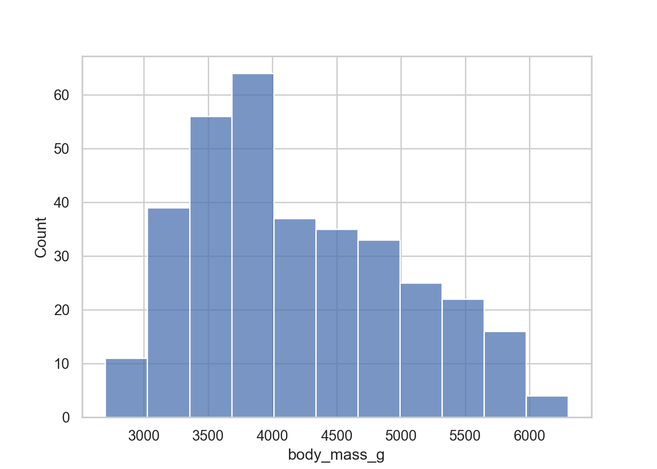
easy enough
sns.histplot(data = penguins, x = "body_mass_g", hue = "species")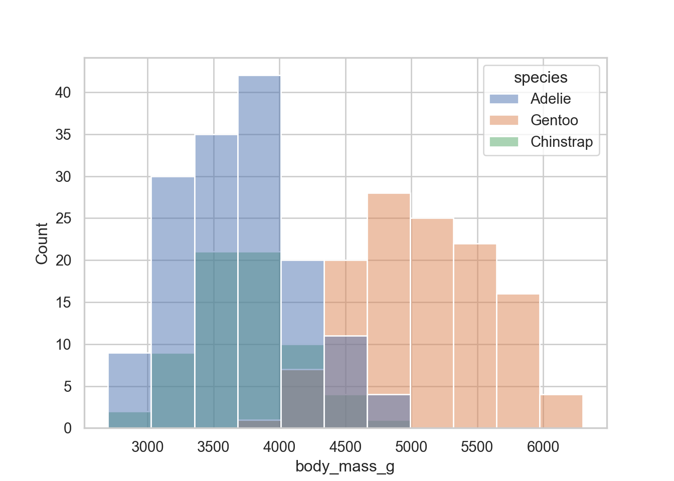
What if we wanted densities instead of frequencies? In ggplot it would be
ggplot(penguins, aes(x = body_mass_g, fill = species)) +
geom_histogram(aes(y =  after_stat(density)))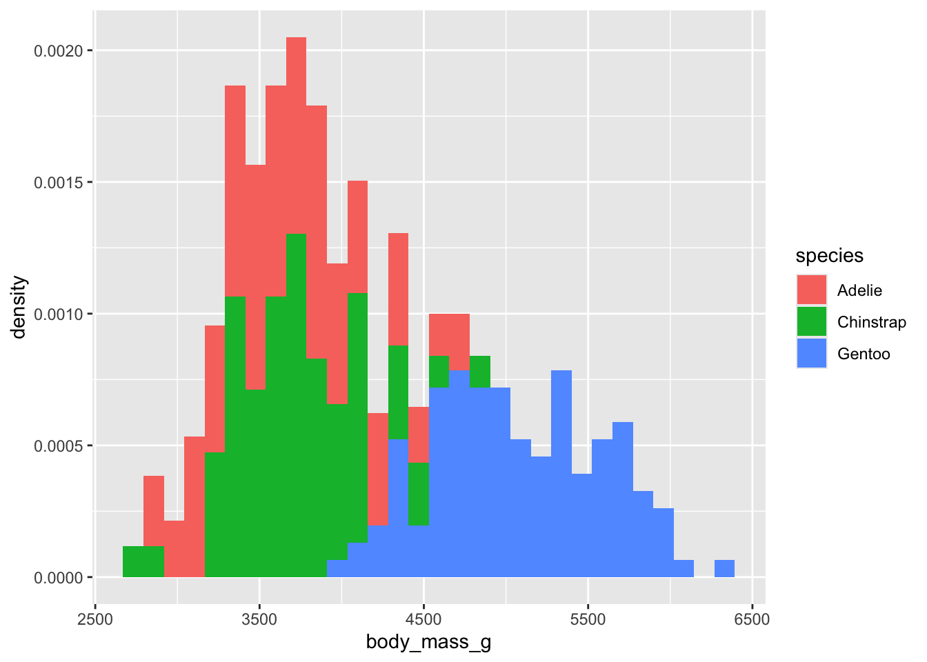
In sns it would be.
sns.histplot(data = penguins, x = "body_mass_g", hue = "species", stat = "density")
I really like the legend on the inside! In new ggplot 3.whatever it is different now that there is an explicit legend.position="inside".
ggplot(penguins, aes(x = body_mass_g, y = after_stat(density), fill = species)) +
geom_histogram() +
theme_minimal() +
theme(legend.position = c(.95,.95),
      legend.justification = c("right", "top"))
Cool I like that and will fiddle with that my ggplot theme!
Okay lets now go and do some bivariate plots. Obviously the workhorse of bivariate plotting is the scatterplot .
Scatter Plots
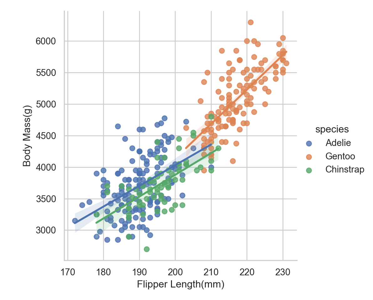
sns.scatterplot(data = penguins, x = "flipper_length_mm", y = "body_mass_g", hue = "species")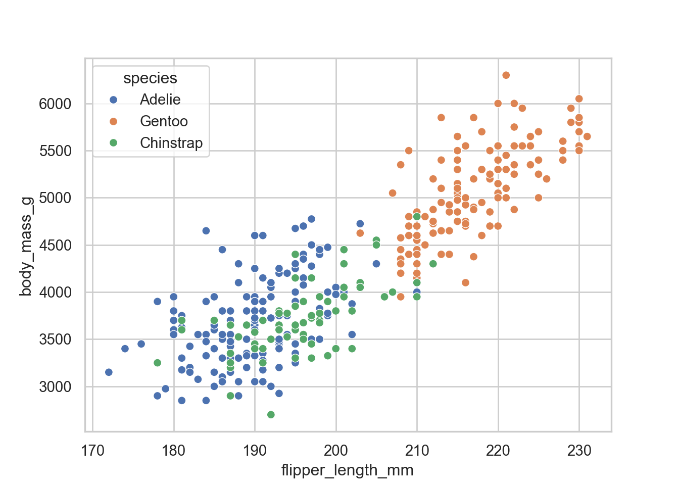
the next thing that we would want is to size points by the size of the penguin
sns.scatterplot(data = penguins, x = "flipper_length_mm", y = "body_mass_g", hue = "species", size = "body_mass_g")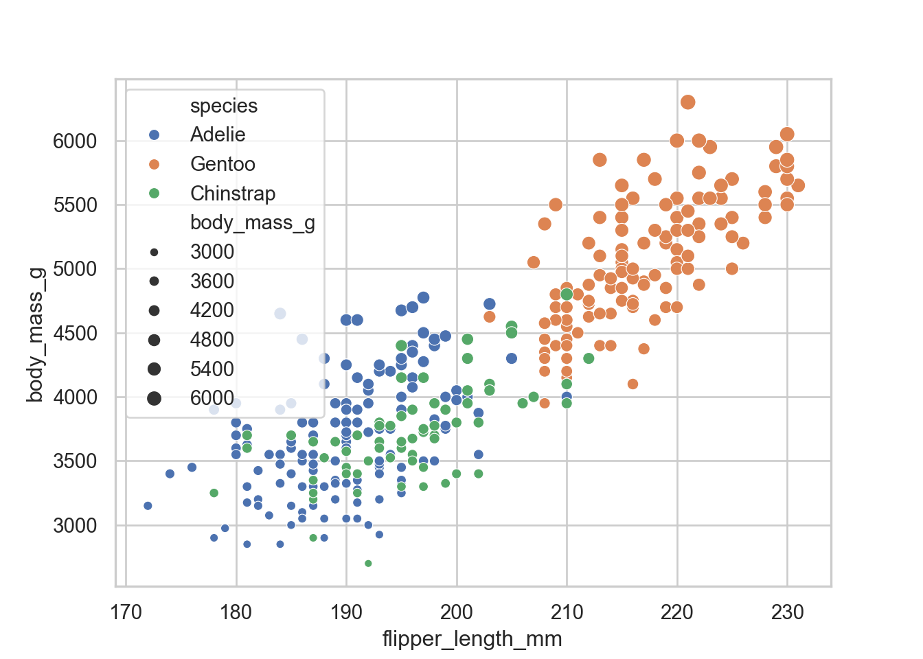
That is not really great since the legend is inside and covering stuff. In ggplot we would simply just move the legend position. In this case we have to save it as an object
Adjusting legend
exmp = sns.scatterplot(data = penguins, x = "flipper_length_mm", y = "body_mass_g", hue = "species", size = "body_mass_g")

sns.move_legend(exmp, "upper left", bbox_to_anchor = (1,1))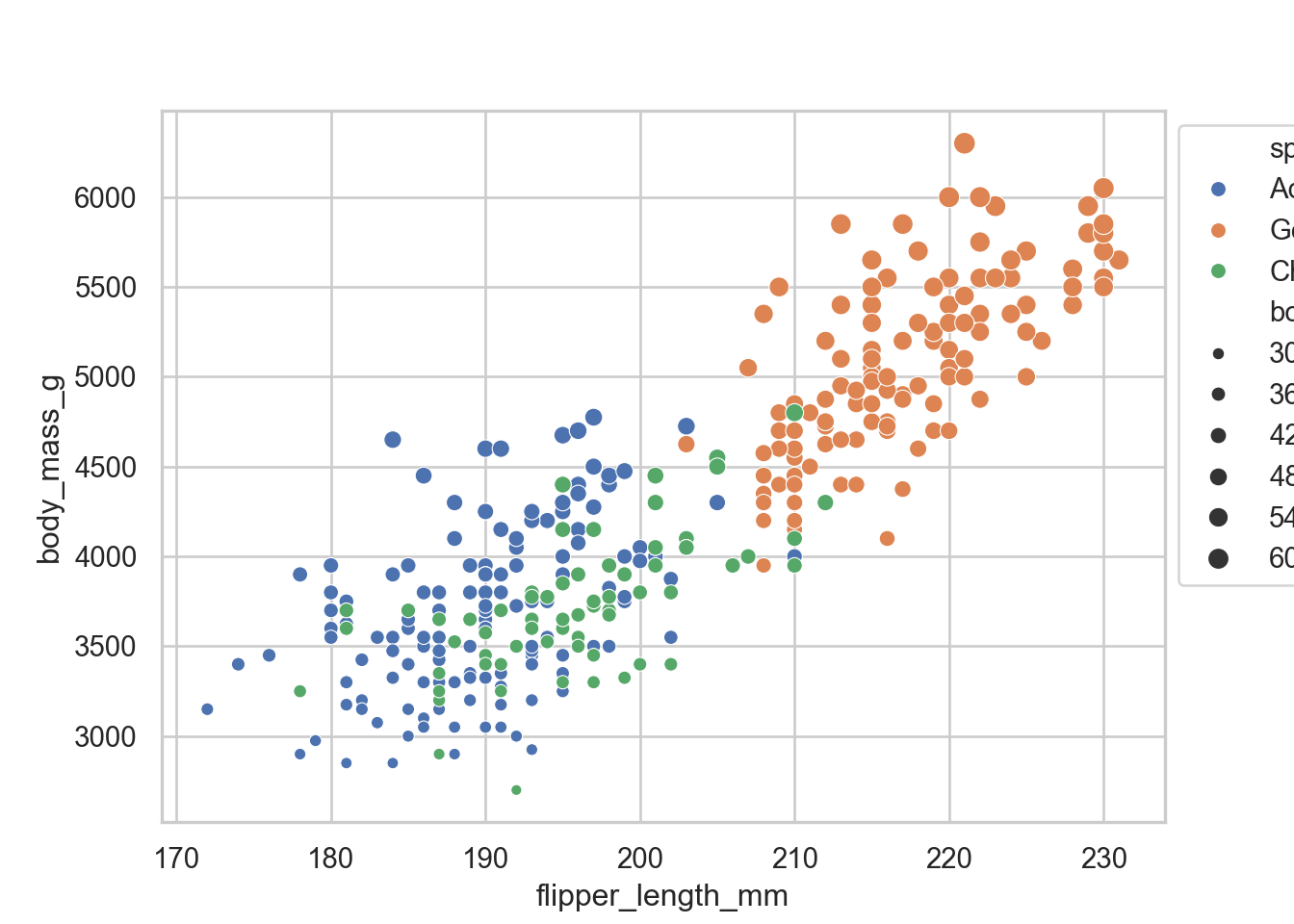
sns.lmplot(data = penguins, x = "flipper_length_mm", y = "body_mass_g", hue = "species")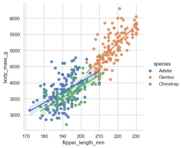
Then the other one that I use all the time is using a line of best fit . Okay obviously the most annoying part is that we don’t have great labels
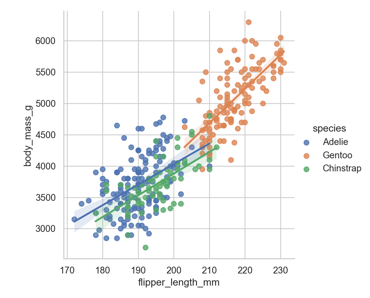
Adding Informative Labels
labs_examp = sns.lmplot(data = penguins, x = "flipper_length_mm", y = "body_mass_g", hue = "species")


labs_examp.set_axis_labels(x_var= "Flipper Length(mm)", y_var = "Body Mass(g)")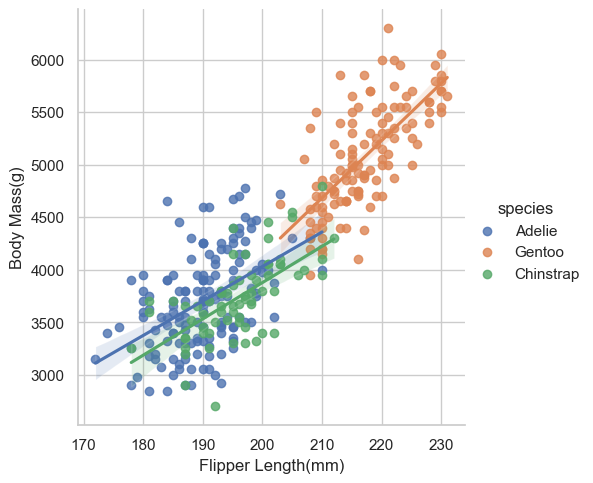
One of the things we may want to do is to create small multiples.
Facet Wrap
sns.displot(data = penguins, x = "body_mass_g", hue = "species", row= "species", facet_kws = dict(margin_titles=False))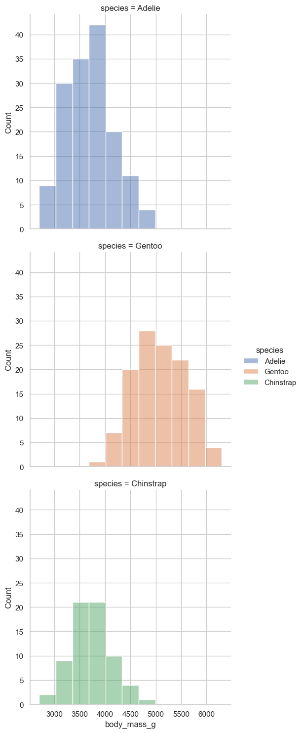
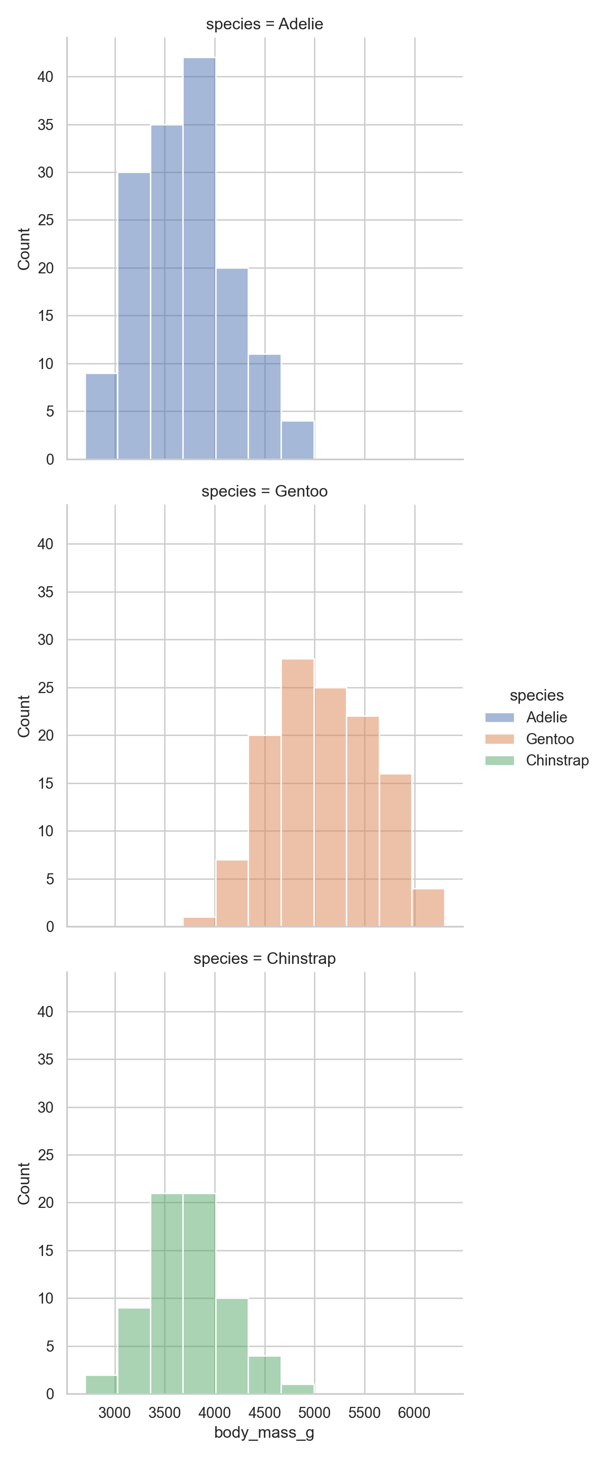
I am honestly not wild about the plot but that is life
Modeling
The last step in the journey is really just learning the basics of modeling. The annoying part is that there is no native support for our favorite stats stuff. So no trusty dust glm or OLS when you open up python. From the excellent marginaleffects package it looks like there is a nice interface called statsmodels and they have a formula api which works like modeling in R just without lazy evaluation.
import statsmodels.formula.api as smf
import numpy as np
Lets fit a few simple models to try and get the hang of statsmodels and see what happens. I will also load broom since I find that it makes working with all the various list components that R spits less annoying to work with.
Lets fit a univariate model first and then we can start playing with the api a little more
library(broom)

naive = lm(body_mass_g ~ flipper_length_mm, data = penguins)

tidy(naive)
# A tibble: 2 × 5
term estimate std.error statistic p.value
<chr> <dbl> <dbl> <dbl> <dbl>
1 (Intercept) -5781. 306. -18.9 5.59e- 55
2 flipper_length_mm 49.7 1.52 32.7 4.37e-107
naive = smf.ols("body_mass_g ~ flipper_length_mm", data = penguins).fit()The biggest difference between the two approaches is that specifying the model and fitting the model are two different steps. If we wanted to see a similar print out we would have to do something like
naive.summary()| Dep. Variable: | body_mass_g | R-squared: | 0.759 |
| Model: | OLS | Adj. R-squared: | 0.758 |
| Method: | Least Squares | F-statistic: | 1071. |
| Date: | Thu, 09 Apr 2026 | Prob (F-statistic): | 4.37e-107 |
| Time: | 13:44:28 | Log-Likelihood: | -2528.4 |
| No. Observations: | 342 | AIC: | 5061. |
| Df Residuals: | 340 | BIC: | 5069. |
| Df Model: | 1 | ||
| Covariance Type: | nonrobust |
| coef | std err | t | P>|t| | [0.025 | 0.975] | |
| Intercept | -5780.8314 | 305.815 | -18.903 | 0.000 | -6382.358 | -5179.305 |
| flipper_length_mm | 49.6856 | 1.518 | 32.722 | 0.000 | 46.699 | 52.672 |
| Omnibus: | 5.634 | Durbin-Watson: | 2.190 |
| Prob(Omnibus): | 0.060 | Jarque-Bera (JB): | 5.585 |
| Skew: | 0.313 | Prob(JB): | 0.0613 |
| Kurtosis: | 3.019 | Cond. No. | 2.89e+03 |
Notes:
[1] Standard Errors assume that the covariance matrix of the errors is correctly specified.
[2] The condition number is large, 2.89e+03. This might indicate that there are
strong multicollinearity or other numerical problems.
Cool. A multivariate model would broadly be the same. One thing that we can do in R is we can transform the predictors in the formula like this
squared = lm(body_mass_g ~ flipper_length_mm + I(flipper_length_mm^2) + bill_depth_mm,
              data = penguins)

tidy(squared)
# A tibble: 4 × 5
term estimate std.error statistic p.value
<chr> <dbl> <dbl> <dbl> <dbl>
1 (Intercept) 16824. 4532. 3.71 0.000240
2 flipper_length_mm -181. 44.9 -4.04 0.0000669
3 I(flipper_length_mm^2) 0.573 0.110 5.19 0.000000363
4 bill_depth_mm 29.3 12.9 2.28 0.0232 We can do something like it.
squared = smf.ols("body_mass_g ~ flipper_length_mm**2 + flipper_length_mm  + bill_depth_mm", data = penguins).fit()


squared.summary()| Dep. Variable: | body_mass_g | R-squared: | 0.761 |
| Model: | OLS | Adj. R-squared: | 0.760 |
| Method: | Least Squares | F-statistic: | 539.8 |
| Date: | Thu, 09 Apr 2026 | Prob (F-statistic): | 4.23e-106 |
| Time: | 13:44:28 | Log-Likelihood: | -2527.0 |
| No. Observations: | 342 | AIC: | 5060. |
| Df Residuals: | 339 | BIC: | 5071. |
| Df Model: | 2 | ||
| Covariance Type: | nonrobust |
| coef | std err | t | P>|t| | [0.025 | 0.975] | |
| Intercept | -6541.9075 | 540.751 | -12.098 | 0.000 | -7605.557 | -5478.258 |
| flipper_length_mm | 51.5414 | 1.865 | 27.635 | 0.000 | 47.873 | 55.210 |
| bill_depth_mm | 22.6341 | 13.280 | 1.704 | 0.089 | -3.488 | 48.756 |
| Omnibus: | 5.490 | Durbin-Watson: | 2.069 |
| Prob(Omnibus): | 0.064 | Jarque-Bera (JB): | 5.361 |
| Skew: | 0.305 | Prob(JB): | 0.0685 |
| Kurtosis: | 3.067 | Cond. No. | 5.14e+03 |
Notes:
[1] Standard Errors assume that the covariance matrix of the errors is correctly specified.
[2] The condition number is large, 5.14e+03. This might indicate that there are
strong multicollinearity or other numerical problems.
However the results differ pretty wildly! Luckily there is an I operator in the underlying thing that makes this work. The problem is that it only works on pandas dataframes
penguins_pd = pd.read_csv('penguins.csv')


squared = smf.ols('body_mass_g ~ I(flipper_length_mm**2) + flipper_length_mm + bill_depth_mm', data = penguins_pd).fit()
Now the results are lining up. As a political scientist by training we love ourselves an interaction term.
interacted = lm(body_mass_g ~ bill_depth_mm * species + flipper_length_mm,
data = penguins)


tidy(interacted)
# A tibble: 7 × 5
term estimate std.error statistic p.value
<chr> <dbl> <dbl> <dbl> <dbl>
1 (Intercept) -4213. 648. -6.50 2.84e-10
2 bill_depth_mm 176. 22.6 7.81 7.22e-14
3 speciesChinstrap 1008. 771. 1.31 1.92e- 1
4 speciesGentoo 129. 608. 0.213 8.32e- 1
5 flipper_length_mm 24.6 3.17 7.76 1.04e-13
6 bill_depth_mm:speciesChinstrap -61.5 42.0 -1.47 1.44e- 1
7 bill_depth_mm:speciesGentoo 78.0 38.5 2.02 4.37e- 2interacted = smf.ols("body_mass_g ~ bill_length_mm * species + flipper_length_mm", data = penguins_pd).fit()
interacted.summary()| Dep. Variable: | body_mass_g | R-squared: | 0.826 |
| Model: | OLS | Adj. R-squared: | 0.823 |
| Method: | Least Squares | F-statistic: | 265.8 |
| Date: | Thu, 09 Apr 2026 | Prob (F-statistic): | 4.07e-124 |
| Time: | 13:44:28 | Log-Likelihood: | -2472.3 |
| No. Observations: | 342 | AIC: | 4959. |
| Df Residuals: | 335 | BIC: | 4985. |
| Df Model: | 6 | ||
| Covariance Type: | nonrobust |
| coef | std err | t | P>|t| | [0.025 | 0.975] | |
| Intercept | -4297.9054 | 645.054 | -6.663 | 0.000 | -5566.772 | -3029.039 |
| species[T.Chinstrap] | 1146.2869 | 726.217 | 1.578 | 0.115 | -282.232 | 2574.806 |
| species[T.Gentoo] | 54.7163 | 619.934 | 0.088 | 0.930 | -1164.739 | 1274.171 |
| bill_length_mm | 72.6920 | 10.642 | 6.831 | 0.000 | 51.759 | 93.625 |
| bill_length_mm:species[T.Chinstrap] | -41.0350 | 16.104 | -2.548 | 0.011 | -72.713 | -9.357 |
| bill_length_mm:species[T.Gentoo] | -1.1626 | 14.436 | -0.081 | 0.936 | -29.559 | 27.234 |
| flipper_length_mm | 27.2632 | 3.175 | 8.586 | 0.000 | 21.017 | 33.509 |
| Omnibus: | 4.761 | Durbin-Watson: | 2.272 |
| Prob(Omnibus): | 0.093 | Jarque-Bera (JB): | 4.564 |
| Skew: | 0.279 | Prob(JB): | 0.102 |
| Kurtosis: | 3.098 | Cond. No. | 1.01e+04 |
Notes:
[1] Standard Errors assume that the covariance matrix of the errors is correctly specified.
[2] The condition number is large, 1.01e+04. This might indicate that there are
strong multicollinearity or other numerical problems.
Again for whatever reason patsy does not have great support for polars dataframe so the original polars frame throws an error.
One thing that we generally want to do is check our OLS assumptions. There are lots of different tests that we can run. But a good first check is to look at the fitted values versus the residuals.
In R we can do
pacman::p_load(patchwork)

dropped_nas = penguins |> drop_na(sex)


with_species = lm(body_mass_g ~ bill_length_mm + flipper_length_mm + species,
             data = dropped_nas)

check_resids = augment(with_species, data = dropped_nas)


violation_one = ggplot(check_resids, aes(x = .fitted, y = .resid, color = species)) +
geom_point() +
theme_minimal()

violation_two = ggplot(check_resids, aes(x = .resid)) +
geom_histogram() +
theme_minimal()


violation_one + violation_two 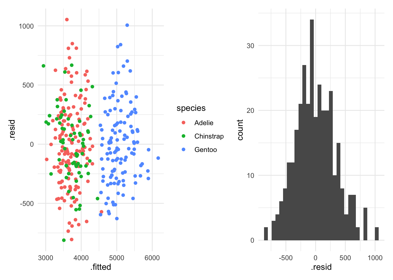
In Python we would do something like this.
penugins_pl = pl.read_csv('penguins.csv')

penguins_sans_na = penguins.filter((pl.col("sex").is_not_null())).to_pandas()


with_species = smf.ols('body_mass_g ~ bill_length_mm + flipper_length_mm + species', data = penguins_sans_na).fit()

penguins_sans_na['fitted_vals'] = with_species.fittedvalues

penguins_sans_na['residuals'] = with_species.resid


sns.scatterplot(x = "fitted_vals", y = "residuals", hue = "species", data = penguins_sans_na)
Misc stuff that are usefull but not neccessarilly useful all the time
Here are the collection of misfits that I thought would be useful
Slice(family)
One useful thing that I use all the time when testing out various things I am doing is using slice. This can be specific rows or a random sample of rows!
If we wanted specific rows we could do this with slice
penguins |>
slice(90:100)
# A tibble: 11 × 8
species island bill_length_mm bill_depth_mm flipper_length_mm body_mass_g
<fct> <fct> <dbl> <dbl> <int> <int>
1 Adelie Dream 38.9 18.8 190 3600
2 Adelie Dream 35.7 18 202 3550
3 Adelie Dream 41.1 18.1 205 4300
4 Adelie Dream 34 17.1 185 3400
5 Adelie Dream 39.6 18.1 186 4450
6 Adelie Dream 36.2 17.3 187 3300
7 Adelie Dream 40.8 18.9 208 4300
8 Adelie Dream 38.1 18.6 190 3700
9 Adelie Dream 40.3 18.5 196 4350
10 Adelie Dream 33.1 16.1 178 2900
11 Adelie Dream 43.2 18.5 192 4100
# ℹ 2 more variables: sex <fct>, year <int>penguins.slice(89:10)invalid syntax (<string>, line 1)It looks like the R user in me strikes. So in polars if you wanted to do the same thing you give the starting number of the row you want and the length of the row you want. So we would rewrite the code like this
penguins |>
slice(90:100)
# A tibble: 11 × 8
species island bill_length_mm bill_depth_mm flipper_length_mm body_mass_g
<fct> <fct> <dbl> <dbl> <int> <int>
1 Adelie Dream 38.9 18.8 190 3600
2 Adelie Dream 35.7 18 202 3550
3 Adelie Dream 41.1 18.1 205 4300
4 Adelie Dream 34 17.1 185 3400
5 Adelie Dream 39.6 18.1 186 4450
6 Adelie Dream 36.2 17.3 187 3300
7 Adelie Dream 40.8 18.9 208 4300
8 Adelie Dream 38.1 18.6 190 3700
9 Adelie Dream 40.3 18.5 196 4350
10 Adelie Dream 33.1 16.1 178 2900
11 Adelie Dream 43.2 18.5 192 4100
# ℹ 2 more variables: sex <fct>, year <int>penguins.slice(89,10)AttributeError: 'DataFrame' object has no attribute 'slice'. Did you mean: 'size'?I actually quite like the syntax of the python version better. It is just annoying having to reset my thinking to start counting at 0
Slice Sample
I find it useful to take a random sample of rows and test functions. It is nice for the function to work on a set of examples you come up with but not everything is consistent so lopping off chunks of a dataset and seeing if it still works is useful.
set.seed(1994)
penguins |>
slice_sample(n = 10)
# A tibble: 10 × 8
species island bill_length_mm bill_depth_mm flipper_length_mm body_mass_g
<fct> <fct> <dbl> <dbl> <int> <int>
1 Chinstrap Dream 50.2 18.7 198 3775
2 Adelie Biscoe 39.7 18.9 184 3550
3 Chinstrap Dream 45.4 18.7 188 3525
4 Gentoo Biscoe 46.2 14.1 217 4375
5 Gentoo Biscoe 50 16.3 230 5700
6 Chinstrap Dream 49.8 17.3 198 3675
7 Adelie Biscoe 35 17.9 192 3725
8 Adelie Biscoe 40.6 18.6 183 3550
9 Adelie Torgers… 40.6 19 199 4000
10 Chinstrap Dream 46.5 17.9 192 3500
# ℹ 2 more variables: sex <fct>, year <int>penguins.sample(n = 10, seed = 1994)TypeError: NDFrame.sample() got an unexpected keyword argument 'seed'Luckily the syntax is broadly the same!
Batch renaming
Often times if we download data from the internet the column names are a mess and we want to rename them all at once. The janitor package in R is extra handy
Lets say we wanted to mass produce a camel case across the entire dataframe. In R that is a fairly simple task. Is it the case for python?
penguins |>
janitor::clean_names(case = "lower_camel")
# A tibble: 344 × 8
species island billLengthMm billDepthMm flipperLengthMm bodyMassG sex year
<fct> <fct> <dbl> <dbl> <int> <int> <fct> <int>
1 Adelie Torge… 39.1 18.7 181 3750 male 2007
2 Adelie Torge… 39.5 17.4 186 3800 fema… 2007
3 Adelie Torge… 40.3 18 195 3250 fema… 2007
4 Adelie Torge… NA NA NA NA <NA> 2007
5 Adelie Torge… 36.7 19.3 193 3450 fema… 2007
6 Adelie Torge… 39.3 20.6 190 3650 male 2007
7 Adelie Torge… 38.9 17.8 181 3625 fema… 2007
8 Adelie Torge… 39.2 19.6 195 4675 male 2007
9 Adelie Torge… 34.1 18.1 193 3475 <NA> 2007
10 Adelie Torge… 42 20.2 190 4250 <NA> 2007
# ℹ 334 more rowsfrom janitor import clean_names
penguins = penguins.rename({"bill_length_mm": "BillLengthMm",
"bill_depth_mm" : "BillDepthMm"})
penguins.clean_names() species island bill_length_mm ... body_mass_g sex year
0 Adelie Torgersen 39.1 ... 3750.0 male 2007
1 Adelie Torgersen 39.5 ... 3800.0 female 2007
2 Adelie Torgersen 40.3 ... 3250.0 female 2007
3 Adelie Torgersen NaN ... NaN NaN 2007
4 Adelie Torgersen 36.7 ... 3450.0 female 2007
.. ... ... ... ... ... ... ...
339 Chinstrap Dream 55.8 ... 4000.0 male 2009
340 Chinstrap Dream 43.5 ... 3400.0 female 2009
341 Chinstrap Dream 49.6 ... 3775.0 male 2009
342 Chinstrap Dream 50.8 ... 4100.0 male 2009
343 Chinstrap Dream 50.2 ... 3775.0 female 2009
[344 rows x 8 columns]In my head it looks like this. Where we are effectively chaining clean names to the dataframe. From the documentation it looks like this
penguins |>
janitor::clean_names(case = "small_camel")
# A tibble: 344 × 8
species island billLengthMm billDepthMm flipperLengthMm bodyMassG sex year
<fct> <fct> <dbl> <dbl> <int> <int> <fct> <int>
1 Adelie Torge… 39.1 18.7 181 3750 male 2007
2 Adelie Torge… 39.5 17.4 186 3800 fema… 2007
3 Adelie Torge… 40.3 18 195 3250 fema… 2007
4 Adelie Torge… NA NA NA NA <NA> 2007
5 Adelie Torge… 36.7 19.3 193 3450 fema… 2007
6 Adelie Torge… 39.3 20.6 190 3650 male 2007
7 Adelie Torge… 38.9 17.8 181 3625 fema… 2007
8 Adelie Torge… 39.2 19.6 195 4675 male 2007
9 Adelie Torge… 34.1 18.1 193 3475 <NA> 2007
10 Adelie Torge… 42 20.2 190 4250 <NA> 2007
# ℹ 334 more rowsclean_names(penguins) species island bill_length_mm ... body_mass_g sex year
0 Adelie Torgersen 39.1 ... 3750.0 male 2007
1 Adelie Torgersen 39.5 ... 3800.0 female 2007
2 Adelie Torgersen 40.3 ... 3250.0 female 2007
3 Adelie Torgersen NaN ... NaN NaN 2007
4 Adelie Torgersen 36.7 ... 3450.0 female 2007
.. ... ... ... ... ... ... ...
339 Chinstrap Dream 55.8 ... 4000.0 male 2009
340 Chinstrap Dream 43.5 ... 3400.0 female 2009
341 Chinstrap Dream 49.6 ... 3775.0 male 2009
342 Chinstrap Dream 50.8 ... 4100.0 male 2009
343 Chinstrap Dream 50.2 ... 3775.0 female 2009
[344 rows x 8 columns]Okay the trick it looks like is that it does not work with polars objects. So we need to pass it to pandas and then back to polars.
import pandas as pd

penguins.glimpse()
Rows: 344
Columns: 8
$ species <str> 'Adelie', 'Adelie', 'Adelie', 'Adelie', 'Adelie', 'Adelie', 'Adelie', 'Adelie', 'Adelie', 'Adelie'
$ island <str> 'Torgersen', 'Torgersen', 'Torgersen', 'Torgersen', 'Torgersen', 'Torgersen', 'Torgersen', 'Torgersen', 'Torgersen', 'Torgersen'
$ bill_length_mm <str> '39.1', '39.5', '40.3', 'NA', '36.7', '39.3', '38.9', '39.2', '34.1', '42'
$ bill_depth_mm <str> '18.7', '17.4', '18', 'NA', '19.3', '20.6', '17.8', '19.6', '18.1', '20.2'
$ flipper_length_mm <str> '181', '186', '195', 'NA', '193', '190', '181', '195', '193', '190'
$ body_mass_g <str> '3750', '3800', '3250', 'NA', '3450', '3650', '3625', '4675', '3475', '4250'
$ sex <str> 'male', 'female', 'female', 'NA', 'female', 'male', 'female', 'male', 'NA', 'NA'
$ year <i64> 2007, 2007, 2007, 2007, 2007, 2007, 2007, 2007, 2007, 2007penguins_pd = penguins.to_pandas()
penguins_clean = clean_names(penguins_pd, case_type = "snake")
penguins = pl.from_pandas(penguins_clean)
penguins.glimpse()Rows: 344
Columns: 8
$ species <str> 'Adelie', 'Adelie', 'Adelie', 'Adelie', 'Adelie', 'Adelie', 'Adelie', 'Adelie', 'Adelie', 'Adelie'
$ island <str> 'Torgersen', 'Torgersen', 'Torgersen', 'Torgersen', 'Torgersen', 'Torgersen', 'Torgersen', 'Torgersen', 'Torgersen', 'Torgersen'
$ bill_length_mm <str> '39.1', '39.5', '40.3', 'NA', '36.7', '39.3', '38.9', '39.2', '34.1', '42'
$ bill_depth_mm <str> '18.7', '17.4', '18', 'NA', '19.3', '20.6', '17.8', '19.6', '18.1', '20.2'
$ flipper_length_mm <str> '181', '186', '195', 'NA', '193', '190', '181', '195', '193', '190'
$ body_mass_g <str> '3750', '3800', '3250', 'NA', '3450', '3650', '3625', '4675', '3475', '4250'
$ sex <str> 'male', 'female', 'female', 'NA', 'female', 'male', 'female', 'male', 'NA', 'NA'
$ year <i64> 2007, 2007, 2007, 2007, 2007, 2007, 2007, 2007, 2007, 2007This works which is awesome! We got back to the original dataset naes
Make a column into a vector
In R there are like a ton of different ways to do this
vec1 = penguins$bill_depth_mm

vec2 = penguins |>
pluck("bill_depth_mm")

vec3 = penguins |>
select(bill_depth_mm) |>
deframe()
In polars the equivalent of this
vec1 = penguins["bill_depth_mm"]

print(vec1[0,1])
shape: (2,)
Series: 'bill_depth_mm' [str]
[
"18.7"
"17.4"
]vec1[1:3][1] 18.7 17.4 18.0import numpy as np
print(vec1[0:2])shape: (2,)
Series: 'bill_depth_mm' [str]
[
"18.7"
"17.4"
]